Bayesian Analysis for Epidemiologists I: Introduction
Acknowledgements
I am indebted to the following individuals upon who’s work the material in these pages has been (extensively) based. I strongly encourage you to follow these links. My notes are really just a pale reflection.
Jim Albert
David Spiegelhalter
Nicky Best
Andrew Gelman
Bendix Carstensen
Lyle Guerrin
Shane Jensen and Statistical Horizons
Contents
I. THE BAYESIAN WAY
1. Why Bayes?
bayes vs. classical
the benefits of bayes
2. Bayes Theorem
example: positive predictive value
example: student sleep habits
II. SINGLE PARAMETER PROBLEMS
1. Single Parameter Binomial Example: Race and Promotion at a State Agency
2. Single Parameter Binomial Example: Perchlorate and Thyroid Tumors
3. Single Parameter Poisson Example: Airline Crashes
4. Single Parameter Normal Model
III. CONJUGATE ANALYSES
1. Conjugate Analysis of Binomial Data
binomial example: drug response
binomial example: placenta previa
2. Conjugate Analysis of Poisson Data
poisson example: London bombings during WWII
poisson example: heart transplant mortality
3. Conjugate Analysis of Normally Distributed Data
example: THM concentrations
IV. PROBABILITY DISTRIBUTIONS USED IN BAYESIAN ANALYSIS
The Bayesian Way
A Bayesian is one who, vaguely expecting to see a horse and catching a glimpse of a donkey, strongly concludes he has seen a mule. (Senn, 1997)
The Bayesian approach is “the explicit use of external evidence in the design, monitoring, analysis, interpretation and reporting of a (scientific investigation)” (Spiegelhalter, 2004)
Bayesian analysis is a natural and coherent way of thinking about science and learning. With advances in theoretical approaches to sampling from marginal and conditional distributions, and the advent of sufficient computing power to make those approaches pragmatic, Bayes is not only theoretically correct, but practical and doable. Some advantages of Bayes are:
- It is flexible and can adapt to complex situations
- It is efficient, using all available information
- It is intuitively informative, providing relevant probability summaries in a way that is consistent with how we think and learn.
- It captures additional uncertainty in predictions by allowing parameter estimates to vary.
In a nutshell, Bayesian inference combines what you observe (the data) with what (you think) you know about the unknown parameters underlying those data. The main difference with classical or frequentist statistics is that in classical statistics, parameters are fixed or non-random, and only the data or samples from the universe of data vary randomly from experiment to experiment. Any inferences on the parameters in which we are interested are couched in somewhat roundabout terms about samples. In Bayesian statistics, unknown quantities like parameters (which we will refer to as \(\theta\)), as well as missing or mis-measured data are treated as random variables and we can make direct probability statements about them.
Since \(\theta\) is a random variable, it has a probability distribution which reflects our uncertainty about it. This is termed the prior distribution (\(Pr[\theta]\)). The data are represented by a probability model termed the likelihood (\(Pr[y|\theta]\)). We use Bayes theorem to combine the prior distribution with the likelihood to obtain the conditional probability distribution for the unobserved quantities of interest given the data, called the posterior distribution (\(Pr[\theta|y]\)). The prior expresses our understanding (or lack thereof) before seeing the data. The Posterior expresses our understanding or the gain in knowledge after seeing the data.
The revolutionary step, actually, is simply expressing uncertainty about parameters with probability distributions. But, as we will see, there is no free lunch. Prior distributions, and how they can reasonably be combined with our data, will complicate our lives. To get a reasonable posterior probability distribution out, you need to put in a reasonable prior opinion concerning the plausibility of values for outcomes like treatment effects.
Why Bayes?
Bayes vs. Classical
Traditionally, statistical analysis has involved four activities intended to answer four questions:
- Estimating unknown parameters (What is the mean value for some medical test in a population?)
- Accounting for variability in estimated parameters (How much does that value vary around the mean?)
- Testing hypotheses (Is the value for the medical test different in treated vs. untreated populations)
- Making predictions (What would we expect the mean value to be in a new sample of patients?)
Classically, parameters (means, standard deviations, regression coefficients, etc…) are considered fixed but unknown. 1 The emphasis is on the sample of data we are using to estimate the parameter. Our estimate of the parameter will change from sample to sample, but it is the samples that vary, not the parameter. This leads to some rather roundabout ways of thinking.
If we believe the only thing varying is the sample, not the underlying parameter, then it behooves us to take many samples and see how those sample estimates of the parameter behave. But this is impractical at best (and nonsensical at worst) under most realistic scenarios. Our data are our data. Rather, we trust in asymptotic theory that if our sample is large enough, the central limit theorem assures us our sample estimate is at or very near the underlying population estimate, and we can adjust our estimates of how it varies from estimate to estimate using the number of observations in the current estimate.
So, while the natural interpretation of a 95% confidence interval is that there is a 95% probability that \(\mu\) is in that interval, that would imply that \(\mu\) varies randomly according to some probability distribution. But, since in the classical framework the the only thing varying is the data or samples, all we can really say is that out of 100 samples, 95 of the samples will contain the true underlying parameter, \(\mu\).
The central philosophical difference between Bayesian vs. classical statistics is that in the Bayesian approach unknown parameters are considered random quantities with their own probability distributions. We are suddenly free of many of the logical gymnastics imposed on us by the classical framework of fixed parameters. But it comes at a cost. In addition to characterizing the probability of the data or sample (which is necessary in both Bayesian and classical approaches) we must now explicitly characterize the probability of the parameters as well. That can get messy.
Both Bayesian and classical statistics involved characterizing the probability or likelihood of the observed data. So, for example, if you are interested in the batting average for a baseball team where each player has an individual batting average, to get the overall probability, you would multiply all the batting averages: \(p(y|\theta = \Pi (y_i|\theta)\). This is termed the likelihood function and is essentially the joint probability of all your observations.
Classical statistics consists primarily of determining the MLE’s for the parameters underlying some set of data. The maximum likelihood estimate involves choosing or determining those parameters that make the data you observed as likely as possible. The details involve taking the derivative of the statistical model (e.g. say a normal probability model) and setting it equal to zero to maximize it. 2 The results are fairly intuitive for standard probability distributions like the normal, where the MLEs that fall out of the calculus are \(\Sigma Y_i/n\) for \(\mu\) and \((y_i - \hat{y})^2/n\) for variance. But they become increasingly more complicated the more complex the data are, and for complex non-standard distributions may be very difficult indeed.
Bayesian statistics also require specifying the MLE’s for the observed data, which is called the data likelihood and can be represent as \(p(y|\theta)\), but now adds the requirement to also specify the unknown parameters \(p(\theta)\), which is called the prior distribution. The general approach is to specify a distribution for the parameters(s) ( the prior), look at data (the likelihood), then combine what we expected with what we observed to update what we think about the parameter (now called the posterior distribution). The updating is done with Bayes rule. We’ll introduce it more formally in a moment, but it is: \(p(\theta|y) = p(y|\theta)p(\theta)/p(y)\), and is usually written as a single line: \(p(\theta|y) \propto p(y|\theta)p(\theta)\) (the \(p(y)\) term is usually dropped because it is there just to normalize or integrate the expression to 1).
The aim of a frequentist approach to, say, a clinical trial is to determine what the trial tells us about the treatment effect. We assume the effect is 0 (\(H_0\)). We collect evidence (data) about this unknown treatment affect, and calculate point estimates, p values, and CI’s as summaries of the size of the treatment effect.
The aim of a Bayesian approach is to learn whether the trial should change our opinion about the treatment effect. To achieve this, we would
- State the plausibility of different values of the treatment effect (the prior distribution)
- State the support for different values of the effect based solely on the trial data (the likelihood)
- Combine these two sources to produce a final opinion about the treatment effect (the posterior distribution)
By combining the prior and the likelihood using Bayes’ Theorem, we are essentially weighting the likelihood or evidence from the trial with the relative plausibilities defined by the prior. It can be viewed as a process of formalized learning from experience. Once you have the posterior distribution, you can get point and interval estimates of treatment effects or any function of the parameters, probabilities of exceeding critical values, predictions for new patients, and prior information for future trials.
This weighting of the posterior and the prior is an essential characteristic of Bayesian analysis. To make this more concrete, consider some normally distributed process, say age in a population. The prior is described by it’s mean and it’s variance around that mean, \(\mu \sim N(\alpha, \tau^2)\). The likelihood is based on a sample of data from the population, is similarly normally distributed (\(y_i \sim N(\mu, \sigma^2)\)) and is described by it’s likelihood, with the MLE for \(\mu\) equal to \(\Sigma y_i/n\) and the MLE for \(\sigma^2\) equal to \((y_i - \hat{y})^2/n\).
According to Bayes Theorem, we can combine the prior, \(p(\theta)\) with the data likelihood \((y|\theta)\) to get at the posterior, \(p(\theta|y)\). If we were to (somehow) know the variance and just had to get at the posterior for the mean, the calculation is:
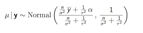
Posterior Distribution for Normal Mean
We can view the posterior distribution as a compromise between the data and the prior The data are represented by how large a sample size you have, \(n\), the prior represented by the standard deviation around \(\mu\) in the prior specification. We will find that this neat analytic calculation is more the exception than the rule. It applies only when standard distributions, like the normal, binomial or Poisson, combine nicely with similar-looking likelihoods. And then, only for simple 1 or perhaps 2 parameter problems. For the far more common and realistic situation, say combining a normal prior with a Poisson likelihood, and resulting distribution would be decidedly non-standard and would require computational approaches.
A lot of the skepticism about Bayesian models comes from the assumptions that go into choosing a prior. Ideally the prior comes from real prior information, which we try to build in to the model in an intelligent and disciplined manner. If though, there is no prior information, or we are not confident in what is known, we can specify a prior that is not too influential. Termed “non-informative” or “minimally informative”, these priors will not weight or update the MLE from the data very much or at all, and the Bayesian results will be identical to the classical results.
The Benefits of Bayes
What then do we gain from the added complications of a Bayesian approach? Most immediately, we will have a probability distribution for the parameter values, so we now we can make direct probability statements about the parameters, and can say things like , “the probability of adding 10 years to life if given drug X is less than 5%”, or “there is a 95% probability that the true value for the effect of drug X is between 5 and 15”. Further, we will not have to rely on asymptotic assumptions. So, even if we don’t have a lot of data, can still do and report an analysis. In this case, the prior will be more influential, so ideally will be based on real and good information, but we can validly evaluate a number of. Finally (and this is the part the most appeals to me) a Bayesian approach allows a principled approach to scientific learning. The forced agnosticism of the classical approach requires us to throw out prior information. But, in the case where we actually have valid and reliable prior information, the Bayesian approach allows us to build it into our analysis.
An additional benefit from a Bayesian approach is in the area of predictions. As noted above, the point estimate for a parameter in the Bayesian framework is simply the mean of the posterior distribution for that parameter. An estimate of variability is calculated as the desired interval from the posterior distribution, with no need to invoke theories about “repeated sampling”. If the estimate of variability contains 95% of the probability in the posterior distribution, it is called the 95% posterior interval or sometimes the 95% credible interval.
We can use the posterior distribution to form the basis for predictions, by specifying the posterior predictive distribution, $ p(y|Y) = p(y|)p(|y)\(, where y* is the value we want to predict, Y is the data, \)(y*|)$ is the new data likelihood, and \(p(\theta|y)\) is the posterior. The Bayesian approach incorporates both the variability in the data (\((y*|\theta)\)) By contrast, the classical approach uses , ignoring variability in \(\theta\). So, for example, in a regression analysis, the classical approach uses a single regression line and predicts using the model. A Bayesian regression model results in a range or distribution of possible regression lines, each with a possible value of \(y*\). As a result, a Bayesian prediction will have more variability around the point estimate.
Bayes Theorem
Bayes Theorem 3, named after the Rev. Thomas Bayes (Turnbridge Wells, England, c1763), is strikingly simple in its derivation, but profound in it’s implications. If you know the probability that A occurs given that B occurs, then Bayes theorem states that we can use that information to calculate the probability that B occurs, given that A occurs. In probability nomenclature, Bayes Theorem says that if we know \(Pr[A|B]\) we can get at \(Pr[B|A]\). We will see that this allows us to ask (and answer) the kinds of questions that really matter, like what is the probability that I have a disease given that I have a positive test (as opposed to what is the probability that my test is positive, given that I have a disease)
Deriving Bayes Theorem is fairly straightforward:
\[ Pr[A \cap B] = Pr[B \cap A] \\ Pr[A \cap B] = Pr[A|B] Pr[B]\\ Pr[B \cap A] = Pr[B|A] Pr[A]\\ Pr[A|B] Pr[B] = Pr[B|A] Pr[A]\\ Pr[A|B] = \frac{Pr[B|A] Pr[A]}{Pr[B]}\\ Pr[B|A] = \frac{Pr[A|B] Pr[B]}{Pr[A]} \]
We are going to pay close attention to the denominator in those last two equations. By the law of total probability, \(Pr[A] = Pr[A|B] Pr[B] + Pr[A|\overline{B}] Pr[\overline{B}]\) , so
\[ Pr[B|A] = \frac{Pr[A|B] Pr[B]}{Pr[A|B] Pr[B] + Pr[A|\overline{B}] Pr[\overline{B}]}\\ Pr[B|A] = \frac{Pr[A|B] Pr[B]}{\sum Pr[A|B] Pr[B]} \]
This equation is for categorical or discrete events, but when we work in probabilities we are frequently interested in probability distributions which sum to one, so the equation may more properly be written:
\[ Pr[B|A] = \frac{Pr[A|B] Pr[B]}{\int dB Pr[A|B]Pr[B]} \]
In terms of parameters and data, Bayes’ theorem is:
\[ Pr[\theta|y] = \frac{Pr[y|\theta] Pr[\theta]}{\int dB Pr[y|\theta]Pr[\theta]} \]
Depending on the situation, this integration in the denominator can be quite difficult or impossible. But all the denominator is doing here is making sure the entire probability integrates to 1, i.e. it is a normalizing factor. The important part for our purposes is the numerator and we find that it is proportional to \(p(y|\theta)p(\theta)\) , i.e. it has the same form, just the overall size changes. You will most often see Bayes Theorem presented in terms of this proportionality, with the denominator left out:
\[ Pr[\theta|y] \propto Pr[y|\theta] Pr[\theta] \]
Example: Positive Predictive Value
The classic example of Bayes Theorem from clinical epidemiology is that of the sensitivity and specificity of a medical test vs. its positive and negative predictive values. in the 1990’s, enzyme-linked immunosorbent assay (ELISA) was used as a screening test for HIV. It was documented as being nearly 100% sensitive and 100% specific for detecting HIV. If the ELISA came back negative, the person was informed they were HIV negative. But, if the ELISA screening test came back positive, a confirmatory Western Blot test was performed. If both the ELISA and the Western Blot were positive, the person was informed they were HIV positive. If the Western Blot was negative, the sample was discarded and person was not informed about their positive screening test.
If, then ELISA was nearly 100% sensitive and specific, why the confirmatory Western Blot for positive screens? Bayes Theorem helps provide the answer
The sensitivity of a screening medical test is the probability that a person will test positive given that they have the disease (\(Pr[+|D\)). The specificity of a test is the probability that a person will test negative given that they do not have the disease (\(Pr[-| \overline{D}\)). But is this really what a patient and his or her healthcare provider are interested? Rather than wondering if they will test positive if they have the disease, they are concerned whether they have the disease given that they tested positive (or don’t have the disease, given that they tested negative). And this, it turns out, is a very different question. These measures are called the positive and negative predictive values of a test. Bayes allows us to answer the question in which we are interested.
Consider the following table of HIV test results. Again, ELISA is the screening test, and Western Blot is the “truth” or “gold standard” that tells us whether someone actually has the disease.
| Western Blot + | Western Blot - | |
|---|---|---|
ELISA + |
498 |
4 |
ELSIA - |
10 |
488 |
Let’s use Bayes Theorem to calculate the sensitivity of the ELISA screening test.4 The sensitivity of a test is the \(Pr[+|D]\) which we can calculate from the table as as:
\[ \frac{Pr[D|+]P[+]}{Pr[D|+]P[+] + Pr[D|-]P[-]}\\ \frac{(498/502)(502/1000)}{(498/502)(502/1000) + (10/498)(498/1000)} \]
In R, we write:
1 | ((498/502)*(502/1000))/(((498/502)*(502/1000)) + ((10/498)*(498/1000))) |
And our result is, as advertised, a sensitivity of 98%.
The calculation for positive predictive value is:
\[ Pr[D|+] = \frac{Pr[+|D]P[D]}{Pr[+|D]P[D] + Pr[+|\overline{D}]P[\overline{D}]}\\ = \frac{(498/508)(508/1000)}{(498/508)(508/1000) + (4/488)(492/1000) } \]
Which results in a positive predictive value of 99%. So, then, why the confirmatory Western Blot? Well, did you notice the prevalence of disease in this population? More than half of this group is HIV positive. In fact, they were a group of IV Drug Users in the New York City area. What if we were to make these calculations with a group with a prevalence more in line with the general population? Since the sensitivity and specificity of a test is an attribute of the test itself, we can apply those proportions to a hypothetical population of a million people, with a disease prevalence of 0.02%:
| Western Blot + | Western Blot - | |
|---|---|---|
ELISA + |
1960 |
9944 |
ELSIA - |
40 |
990056 |
A positive predictive value using these numbers is:
\[ \frac{(1960/2000)(2000/1000000)}{(1960/2000)(2000/1000000) + (784/998000)(998000/1000000)} \]
For a positive predictive value of about 20%.
We can see a couple of things here. First, Bayes Theorem works, and that’s certainly nice enough. Second, we can use Bayes theorem to derive probabilities for separate but related events, and that’s actually quite provocative. Third, some terms we use in epidemiology, like prevalence, may have different names, like \(Pr[D]\) in other statistical traditions. That is only to be expected, but can pose an initial obstacle to understanding Bayesian statistics.
This use of Bayesian analysis is well-accepted and uncontroversial. It’s been said a frequentist is someone who only uses Bayes Theorem sometimes. The controversy arises when extending these principles to general statistical analysis, where parameters are assigned probability distributions.
Example: Student Sleep Habits
As a first Bayesian analysis, Jim Albert considers the proportion of college students who get more than 8 hours sleep. His intuition tells him it is about 30%. He surveyed one of his classes and found that 11 of 27 (47%) had slept more than 8 hours the night before. What would the Rev. Bayes say about this? That we need to update our prior assumptions in light of the data, and that we can calculate a new (posterior) probability distribution proportional to the product of our initial assumptions (prior) and the data (likelihood):
\[ posterior \; \propto \; prior \; * \; likelihood \\ p(\theta | y) \propto p(\theta)*p(y | \theta) \]
The data (our likelihood) is binomially distributed as \(\theta^k * (1-\theta)^{n-k}\), where \(\theta\) is the probability of sleeping more than 8 hours, \(k\) is the number of students who said they slept more than 8 hours, and \(n\) is the number of students surveyed.
The prior is a bit more difficult to nail down. Say we believe \(\theta\) is somewhere between 0 and 50%, but mostly clustered around 30%. We’ll need to specify it a bit more precisely. There are a couple of ways to do that. We will most often define a continuous probability distribution to describe our prior assumptions, but in this first simple case, let’s take a so-called “discrete” approach. This involves writing a list of plausible values, weighting them by how probable we think they are, and then converting the weights to a probability distribution that sums to one by dividing through by the sum of the weights.
- plausible values for proportion of heavy sleepers (theta)
- 0.05, 0.15, 0.25, 0.35, 0.45, 0.55, 0.65, 0.75, 0.86, 0.95
- weights for those plausible values
- 0, 1, 2, 3, 4, 2, 1, 0, 0, 0
- convert to probabilities
- 0.00, 0.08, 0.15, 0.23, 0.31, 0.15, 0.08, 0.00, 0.00, 0.00
To calculate the posterior, we multiply each value of the posterior by the likelihood of that value. The actual calculations involve log transformations and some other manipulations. Jim Albert’s “LearnBayes” package has a function called pdisc(), that makes the calculations relatively straightforward. Let’s load the package and find out a little about pdisc().
1 2 | library(LearnBayes)
?pdisc |
First, we assign our likelihood data to an object called (appropriately enough) “data”. Then we create our prior and plot it.
1 2 3 4 5 6 | data<-c(11, 16) # number successes and failures theta<-seq(0.05, 0.95, by = 0.1) weights<-c(0, 1, 2, 3, 4, 2, 1, 0, 0,0) prior<-weights/sum(weights) plot(theta, prior, type="h", ylab="Prior Probability") |
Now, we use the pdisc() function to calculate the posterior, and then print a table of the
1 2 | post<-pdisc(theta, prior, data) round(cbind(theta, prior, post), 2) |
And now a little plot to see how our prior has changed or been updated in light of the data.
1 2 3 4 5 6 7 8 9 | par.old<-par() par(mfrow=c(3,1)) plot(c(0,1),c(11/(11+16),16/(11+16)), type="h", ylim=c(0,.7), lwd=5, main="data" ) plot(theta, prior, type="h", ylab="Prior Probability", ylim=c(0,.7), lwd=5, main="prior") plot(theta, post, type="h", ylab="Posterior Probability", ylim=c(0,.7), lwd=5, main="posterior") par(par.old) |
This plot, from Jim Albert’s book, more clearly illustrates the prior and the posterior.
Discrete Prior to Discrete Posterior
In the following sections we explore the process of updating our prior distribution for various kinds of parameters by combining it with evidence from a data likelihood to produce a posterior distribution.
Single-Parameter Problems
As with most introductions to Bayesian analyses we begin with relatively simpler single parameter problems, like trying to estimate the single underlying proportion in a binomial problem, or the single underlying rate in a Poisson model, or (less realistically) the mean in a normal model where we already know the standard deviation. 5 These problems can be solved analytically, i.e. there are formulas to combine a prior with a likelihood to get at a reasonable specification for a posterior. We will explore how and why these analyses “work” in the following section on conjugate analyses, but for now will simply present some early examples.
Single Parameter Binomial Example: Race and Promotion at a State Agency
In a state agency, 26 of 48 blacks or African Americans passed a test for promotion, compared to 206 of 259 White applicants. Proportions like these have a binomial data likelihood. If we have no previous evidence or information upon which to base a prior distribution, we may use a minimally or non-informative prior. In this case (for reasons that will be come clearer when we go through the discussion of conjugate analyses in the next section) a Beta distribution will work well. In this case we use a Beta(1,1) distribution which is flat on range from 0 to 1 and results in a non-informative uniform prior. The Beta(\(\alpha\), \(beta\)) distribution is flexible, if \(\alpha\) = \(beta\), it is uniform, if \(\alpha\) {} \(beta\), humped to right, if \(\alpha\) {} \(beta\), it is humped to the left. (See the section below on probability distributions.)
We can combine the binomial likelihood with the Beta prior in simple analytic fashion: mathematically just add the Beta \(\alpha\) parameter from the prior to the number of successes from the binomial data likelihood, then add the Beta \(\beta\) parameter from the prior to the number of failures, which will results in a Beta(\(y+\alpha\) , \(n-y+\betab\))) posterior. In this example then, the resulting posterior distribution for the Black applicants is Beta(27,23). We repeat this process for the data from White applicants for a Beta (207,54) posterior distribution. We then simulate or sample from these two distributions many times, and compare the two samples to draw inferences.
Here is the code for this procedure:
1 2 3 4 5 6 7 8 9 10 11 12 13 14 15 16 17 18 19 20 21 22 23 24 25 26 27 28 29 30 31 32 33 34 35 36 37 38 39 40 41 42 43 | # data y.black <- 26; n.black <- 48 y.white <- 206; n.white <- 259 # likelihood for black applicants ?rbinom likelihood.black<-rbinom(10000, 48 ,(26/48)) plot(density(likelihood.black)) # Beta(1,1) prior ?rbeta prior<- rbeta(10000,1,1) plot(density(prior)) # posterior from updated uniform Beta(1,1) by adding 1 to number # of successes and 1 to number of failures # 10000 simulation for blacks and whites theta.black <- rbeta(10000,y.black+1,n.black-y.black+1) theta.white <- rbeta(10000,y.white+1,n.white-y.white+1) # plot densities old.par<-par() par(mfrow=c(2,1)) plot(density(theta.black), xlim=c(0,1), main="probability blacks passing") plot(density(theta.white), col="red", xlim=c(0,1), main="probability whites passing") # plot histograms mintheta <- min(theta.black,theta.white) maxtheta <- max(theta.black,theta.white) hist(theta.black,col="gray",xlim=c(mintheta,maxtheta)) hist(theta.white,col="gray",xlim=c(mintheta,maxtheta)) par(old.par) # compute posterior probability blacks scoring less than whites # proportion times in 10000 simulations blacks scored less than whites (prob <- sum(theta.black <= theta.white)/10000) # essentially 100% |
We can extend this model to predict how many African American applicants from among 100 future applicants would be expected to pass this test. Again, in addition to the variation in the data (the likelihood) we will add the variation in the underlying parameter (\(\theta\)) The process involves 1)sample a large number (10000) of \(\theta\)’s from the Beta(27,23) posterior, then 2)for each of those values of \(\theta_i\), sample a single y* from Binomial(100, \(\theta_i\)). By contrast, a classical approach might be a parametric bootstrap, sampling y* from Binomial(100, \(\theta\)) from single value of \(\theta\)
A couple of points about the prior in this analysis. First, note that the uniform Beta(1,1) prior subtly pulls the posterior estimate to the middle. We will see that this kind of compromise between the data and the prior is one of the defining characteristics of Bayesian analysis. The influence of the prior, in fact, allows us to draw some conclusions in sparse data settings when classical approaches are not possible. For example, say there are zero outcomes in some sample. In the classical framework, the CI of 1.96 plus minus \(\sqrt{pq/n}\) collapses to 0 plus or minus 0. The Bayesian approach allows some estimation, e.g we can apply an uninformative Beta(1,1) to a Binomial (0, 25) likelihood to arrive at a Beta(1,26) posterior. With the \(\alpha\) term so much less than the \(\beta\) term we would expect almost all the probability to be humped up on the left side of the curve near zero. But it does return a result.
Second, while a uniform or flat prior on 0 to 1 is indeed only minimally informative, and makes sense in this binomial setting, it might not in other settings. Consider, for example, a normal prior for the mean of a normally distributed likelihood. A flat prior would go from minus infinity to plus infinity. Do we really know so little about the mean that we think it can be anything at all? Ranging infinitely? As a general rule, you should evaluate the sensitivity of your results to your prior specification. For small data sets (say 5 or six observations) the choice of prior will invariable be influential. For more reasonably-sized data sets,the results will be more robust, but you should still look at how they behave for different specification of a prior.
In the 1950’s Sir Harold Jeffreys described an approach or general scheme for selecting minimally informative priors that now bears his name. It involves setting the prior equal to the square root of the expected Fisher information (you can see the details here). The Jeffreys prior for binomial data is Beta(0.5,0.5) for \(\theta\)
Single Parameter Binomial Example: Perchlorate and Thyroid Tumors
Let’s look at another single parameter binomial problem as a motivating example. In this case we’ll look at little more closely at how in the setting of sparse data, a Bayesian approach can help us draw inferences when a classical approach might not, and how a more informative prior could help us advance and update our thinking about a problem . This data for this example comes from an online presentation by David Dunson at the US National Institute for Environmental Health Sciences.
Percholorate is a ground water contaminant that has been associated with thyroid tumors. In a study, 2 of 30 lab rats exposed to perchlorate developed thyroid tumors, compared to 0 of 30 control rats. What conclusions can be draw? Given the small numbers, a first reasonable approach in the classical framework might be a Fisher’s exact test.
{.r .numberLines} (rat.dat<-matrix(c(2,0,28,30), nrow = 2)) fisher.test(rat.dat)
The p-value is 0.49, indicating no association, but as noted above, because of the zero value, the confidence interval collapses to infinity. What can we learn from a Bayesian approach? Let’s repeat our approach to binomial data from above
1 2 3 4 5 6 7 8 9 10 11 12 13 14 | # data y.perchlorate <- 2; n.perchlorate <- 30 y.control <- 0; n.control<- 30 # update Beta(1,1) prior for exposed and unexposed theta.perchlorate <- rbeta(10000,y.perchlorate+1,n.perchlorate-y.perchlorate+1) theta.control <- rbeta(10000,y.control+1,n.control-y.control+1) # graphically compare exposed and unexposed par(mfrow=c(2,1)) plot(density(theta.perchlorate), xlim=c(0,1), main="probability of tumor in exposed rats") plot(density(theta.control), col="red", xlim=c(0,1), main="probability of tumor in control rats") # probability that exposed have more tumors than unexposed sum(theta.perchlorate >= theta.control)/10000 |
We find that the Beta(1,1) prior exerts considerable influence on these analyses. In fact, we can interpret it as corresponding to having as much information as two observations, one with the outcome, and one without. In this case, adding that information indicates that in 87% of the simulations, perchlorate exposed rats developed more thyroid tumors than control rats. This is a very different conclusion than from the classical analysis. Let’s go a bit further. What is the difference in the number of tumors between these two groups of rats? In a Bayesian framework it is as simple as subtracting one set of simulations from the other and examining the resulting distribution.
1 2 3 4 5 | theta.diff<-theta.perchlorate-theta.control # 95% credible interval quantile(theta.diff, probs=c(0.05,0.95)) # plot differences plot(density(theta.diff)) |
We see that now, as opposed to the classical approach, we can calculate a 95% interval for the difference in tumors between the two groups of rats. It includes zero, so it is consistent with the non-significant classical p-value from the Fisher’s exact test. But we also see that the majority of the probability lies above zero, which reflects our probability calculation above. It is reasonable to continue to be concerned about the association of perchlorate with tumors.
An additional advantage of a Bayesian approach can be seen if we have some real prior evidence or belief about the putative association of perchlorate and thyroid tumors. It would be reasonable to assume that we do. Why else would we be doing this experiment in the first place? Dr. Dunson, in his presentation, suggests a Beta(0.11, 2.6) as representing previous experimental evidence. Let’s use that prior, and combine it with our data to update the posterior.
1 2 3 4 5 | theta.perchlorate <- rbeta(10000,y.perchlorate+.11, n.perchlorate-y.perchlorate+2.6) theta.control <- rbeta(10000,y.control+.11,n.control-y.control+2.6) theta.diff<-theta.perchlorate-theta.control quantile(theta.diff, probs=c(0.05,0.95)) |
And, in fact, taking what we know about the topic into account, pushes our 95% interval for the difference between the exposed and unexposed rats out of the range of zero.
Single-Parameter Poisson Example: Airline Crashes
As in the case of a binomial data likelihood combined with a Beta prior distribution, there is a relatively straightforward (at least when you see the end result…) analytic solution to the setting when there is a Poisson likelihood of count data. It turns out that a Poisson data likelihood combines nicely with a Gamma prior to produce a Gamma posterior.
This example again comes from Dr. Shane Jensen. Consider the count of airline crashes per year over a 10-year period form 1976 to 1985: \(y = (24, 25, 31, 31, 22, 21, 26, 20, 16, 22)\). Note that now, as opposed to the setting of binomial data, which are the number of events or “successes” that occur out of some total number of opportunities, we don’t have the underlying number of opportunities. 6. What we do have, is 10 realizations of a poisson process with some underlying rate that (importantly) does not change over those 10 realizations. the results are interpreted as the rate of crashes. (We’ll address the issue of whether it is reasonable to assume an unchanging rate over time shortly.)
Each year of data is distributed as \(p(y_i|\theta) \theta^{y_i}e^{-\theta}/ y_i!\). We multiply the probability of each year of data to get likelihood of the data: \(p(y|\theta)=\theta ^{\Sigma y_i}e^{n\theta}/\Pi y_i!\). An analytically convenient prior is the Gamma distribution, which is also a series of realizations on the positive real line and (more importantly) has the same functional form as Poisson does (\(\theta^{\alpha - 1} e^{-beta * \theta}\)). You can, roughly, think of this analytic convenience as due to the two distributions looking similar to each other. The analytic solution for the posterior distribution when we have a Poisson data likelihood and a Gamma prior is \(Gamma(y_i + \alpha, n + \beta)\)
Again, as in the binomial case, we can interpret the influence of the Gamma prior parameters \(\alpha\) and \(\beta\) in terms of our data. Here, \(n\) is number of years of data, so can think of the \(\beta\) term as the “number of years of data” that we believe our prior is worth, and \(\alpha\) is the number of outcomes we believe our prior is worth. The mean of the Gamma is \(a/b\), so the mean of the posterior is \(\frac{y_i + \alpha}{n + \beta}\) and we can again see the resulting prior as a compromise between our data and the prior. The minimally informative Jeffrey’s prior for this setting is Gamma(0.5,0), which is improper, so we use Gamma(0.5,0.0001). Here is some code to run this example.
1 2 3 4 5 6 7 8 9 10 11 12 13 14 15 16 17 18 19 20 21 22 23 24 25 26 27 28 29 30 31 32 33 34 | # data years <- c(1976,1977,1978,1979,1980,1981,1982,1983,1984,1985) crashes <- c(24,25,31,31,22,21,26,20,16,22) numyears <- length(years) sumcrashes <- sum(crashes) # posterior from updated non informative (Jeffrey) prior theta <- rgamma(10000,shape=(sumcrashes+0.5),rate=(numyears+0.0001)) plot(density(theta)) # posterior predictive distribution for crashes in next year y.star <- rep(NA,10000) # vector to hold simulations # sample one observation from the posterior distribution for (i in 1:10000){ y.star[i] <- rpois(1,theta[i]) } # plot histograms for data, posterior and posterior predictive on same scale par(mfrow=c(3,1)) hist(crashes,col="gray",xlim=c(0,50),breaks=10) hist(theta,col="gray",xlim=c(0,50)) hist(y.star,col="gray",xlim=c(0,50)) posterior distribution vs. the posterior predictive distribution mean(theta) quantile(theta, probs=c(0.05,0.95)) mean(y.star) quantile(y.star, probs=c(0.05,0.95)) sum(theta>30)/10000 sum(y.star>30)/10000 |
We are extending the approach to simulate the posterior predictive distribution. Recall, that this includes both the variation in the data and the variation in the rate parameter. (As opposed to classical predictions that include only the variation in the data.) We can see both graphically an in the 95% probability intervals how much more variation goes into the posterior predictive. We can also see that there is a 10% probability that crashes in the following year will exceed 30.
Single-Parameter Normal Model
As we saw above, a single parameter version of the normal model exists, though it doesn’t make a lot of practical sense because it assumes we don’t know the mean, but somehow do know the variance. The most analytically tractable prior distribution for a normal data likelihood turn out to be, in fact, the normal distribution itself. 7 The resulting posterior is also normal.
Posterior Distribution for Normal Mean (\(\alpha\) = prior mean, \(\mu_0\))
Again, can see that a small value of \(\tau\) up weights the prior value for the mean (\(\mu_0\)). Alternatively as data accumulate and \(n\) increases, the posterior has to move toward the data likelihood. The posterior in the normal setting, then, is “controlled” by 3 things: how noisy the data are, confidence in our prior (\(\tau\)), and how much data we have (\(n\)). We have 2 main ways of making the data more influential: get more data, or make \(\tau\) much bigger. A normal prior with infinite variance approaches a flat distribution as its limit, and is, in fact, the Jeffreys prior for the normal setting, though it is improper, and (again) infinite variance may not make much sense. We also note that by setting \(\tau\) to infinity, posterior ends up being \(\sim Normal(\hat{y}, \sigma^2/n)\) which is, in fact, what we see in classical statistics as result of MLE (e.g. CI $ +1.96* / $)
And, again, when making predictions, the classical approach would involve a calculation for a single \(\bar{y}\) with variability, a Bayesian would put in additional variability from choice of potential \(\bar{y_i}\).
Conjugate Analyses
In the previous section we spent time working with what are termed conjugate priors. In this section we’ll further explore and expand those types of Bayesian analysis, which are useful in their right, but also introduce important concepts underlying the Bayesian framework.
Conjugacy refers to a statistical relationship between probability distributions, in this case the prior distribution, the likelihood and the posterior distribution. A prior is said to be conjugate to a likelihood if both the prior and the likelihood are in the same statistical “family” or class of parametric densities. Combining a conjugate prior and likelihood results in a posterior that is the same type of distribution as the prior. We have already seen that a beta prior distribution combines with a binomial likelihood to produce an updated beta posterior. Also, that a gamma prior is conjugate to a Poisson likelihood and results in a gamma posterior. The last class of conjugacy (which we haven’t yet explored) is the combination of a normal prior with a normal likelihood for a normal posterior.
In the simplest cases of one, or perhaps two, parameters, we can combine conjugate priors and likelihoods analytically. We have already seen how simple it is to update a beta or gamma prior by adding terms to the specification of the likelihood. For relatively simple problems, this might be all that we need. But we will quickly run into problems with more realistic situations for which there are no simple analytic solutions. In those situations (which we will explore in future sections) we will have to rely on computational approaches that involve sampling from the proposed posterior distribution. This sampling may be simple, or more complex involving concepts like Markov Chain Monte Carlo using Metropolis-Hastings or Gibbs sampling.
For now, we will use the relatively simpler setting of conjugate analysis to introduce some tools and concepts we will use for more complex future analyses.
| Likelihood | Prior | Posterior |
|---|---|---|
Normal |
Normal |
Normal |
Binomial |
Beta |
Beta |
Poisson |
Gamma |
Gamma |
Conjugate priors are mathematically convenient, but don’t exist for all likelihoods. Computations for non-conjugate priors are at best difficult and at worst intractable. The advent of MCMC, i.e BUGS, removed these restrictions. It is still, though, useful and appropriate to have some knowledge of conjugate analyses if only because most MCMC software still uses them when available and appropriate, to speed up analyses.
Conjugate Analysis of Binomial Data
A lot of epidemiology involves binomial data such as proportions and risk estimates, so we begin with and spend some additional time on the topic. The data likelihood (\(Pr(y | \theta)\)) for binomially distributed data is described as k “successes” or responses out of n trials or observations. The binomial probability distribution is \(\binom{n}{k} p^k q^{n-k}\) where \(p\) is the probability of the event occurring in a single trial, \(q\) is the probability of the event not occurring (\(1-p\) by the complement rule) and \(\binom{n}{k}\) is the binomial expansion ’’n choose k" the formula for which is: \(\frac{n!}{k!(n-k)!}\) 8
In this example, then, \(q\) is the parameter \(\theta\) in which we are interested. Our prior distribution (\(Pr(\theta)\)) describes how we think \(\theta\) varies, or the values \(\theta\) may take and how likely they are. If we think all values of \(\theta\) are equally likely, we can use a uniform prior, which, as we have seen, we can achieve with a \(\sim Beta(1,1)\). By Bayes’ Theorem, the posterior distribution which combines our prior and our likelihood is:
\[ Pr(\theta|y) = Pr(\theta | k, n) \propto (\theta^k)(1-\theta)^{n-k}*1 \]
It turns out that with a \(\sim Beta(a,b)\) prior, the posterior is also a Beta distribution:
\[ Beta(a+k,b+n-k) \]
Which in this case is
\[ \sim Beta(1+k, 1+n-k) \]
We can use this distribution to assess the outcome in terms of means, medians and probability intervals.9
Binomial Example: Drug Response
Say we are interested in the response of patients to a drug. We believe somewhere between 0.2 and 0.6 of patients will respond, with a mean of 0.4 and a sd=0.1. In a study of 20 persons, what is the probability that 15 will respond? A Beta(9.2, 13.8) distribution will fit these parameters (we will see where this came from in a moment).
It is straightforward to code this up in R. We start by running 1,000 simulations for the parameter using the rbeta() function, then feeding those simulations to a the rbinom() function to create a set of examples. We then plot the density and calculate the probability of a result greater than 15 successes.
1 2 3 4 5 6 7 | N=1000 theta<-rbeta(N,9.2,13.8) x<-rbinom(N,20, theta) y<-0 accept<-ifelse(x>14.5, y+1, y+0) plot(density(accept)) (prob<-sum(accept)/N) |
As a an aside, we will soon be running models in programs like WinBUGS and JAGS. As a quick preview, here is what the model code would look like in one of those programs:
1 2 3 4 5 6 | #binomial monte carlo Model{ y~dbin(theta , 20) #sampling distribution theta ~ dbeta (9.2, 13.8) #parameter from sampling distribution p.crit <- step(y-14.5) # indicator variable, 1 if y>=15, 0 otherwise } |
However we run the simulation, the probability is about 1.5%. Note that this answer is pure simulation or Monte Carlo, we have not (yet) included any data. We are simply drawing random samples from a distribution. Suppose that we enroll and treat 20 volunteers and 15 of them respond to the treatment? Let’s use a conjugate analysis to determine how our prior is updated to a posterior probability of the the effectiveness of the drug given these data.
Analysis With Data for the Likelihood
Our prior probability is still a Beta (9.2, 13.8) density. But now that we have data, we have a likelihood. Here, the binomial probability of observing 15 successes in 20 trials. Using the conjugate approach, we update the Beta(9.2, 13.8) to a Beta (9.2+15, 13.8+20-15) = Beta (24.2, 18.8) which has a \(\mu\) =24.2/24.2+18.8 = 0.56. Basically, we are taking the Beta (9.2, 13.8) probability distribution, combining it with the Binomial likelihood probability distribution of observing 15 success in 20 trials and coming up with a new, updated, Beta distribution as our posterior. We have already seen this kind of analysis when considering the proportion of African American applicants who succeeded on a promotion test, and when looking at the proportion of lab rats that developed thyroid tumors when exposed to a toxin.
1 2 | theta.drug<-rbeta(10000, 24.2, 18.8) mean(theta.drug) # check mean close to analytic |
Now, suppose we are considering further development of the drug. We decide that if we see at least 25 further successes out of 40 additional patients we will continue funding drug development. How likely it be to observe 25 successes in another 40 patients? Let’s predict by by using the posterior distribution as the prior.
1 2 3 4 5 | x<-rbinom(N,40, theta.drug) y<-0 accept<-ifelse(x>24.5, y+1, y+0) prob<-sum(accept)/N prob |
The probability for \(k>25\) is about 33%.
Sneak Peak at Running an MCMC Model
Let’s take a moment to see how a similar analysis might be done in one of the Markov Chain Monte Carlo (MCMC) Gibbs sampler programs we will be talking a lot more about soon. In this case we’ll be using JAGS (Just Another Gibbs Sampler). The beauty of sampling algorithms like those found in WinBUGS and JAGS is that we don’t have to be constrained to the simple situations where closed (conjugate) forms are available. Using MCMC, there is no need to explicitly specify the posterior like we do when, say, we add the Beta parameters to the Binomial likelihood. These programs have algorithms to evaluate the posterior given (almost) arbitrary specification of the prior and the likelihood. Although it’s worth noting that programs like WinBUGS and JAGS will look for conjugacy and use it if it exists. Let’s look at the the JAGS syntax for this drug investigation example.
We begin by writing up the model code.
1 2 3 4 5 6 7 8 9 | cat( "model { y~dbin(theta, m) #likelihood theta~dbeta(a,b) # prior y.pred~dbin(theta, n) #posterior, used as predictive distribution p.crit<- step(y.pred-ncrit+0.5) # if y.pred>=ncrit, returns 1, otherwise 0 }" ,file="m1.jag") |
Next, we specify the data for the beta parameters, the number of trials for the likelihood and for the prediction. Note that in WinBUGS, we could write these data values into the model statement itself, but the more common approach (and one required by R2WinBUGS and R2jags) is to specify the data separately.
1 2 3 4 5 6 | m1.dat<-list(a=9.2, b=13.8, y=15, m=20, n=40, ncrit=25) |
Now, we run the model in JAGS, using the R2jags package to interface with the Gibbs sampler, and explore the results using both the default “rjags” object, and converting to an “mcmc” object so we can use the coda package.
1 2 3 4 5 6 7 8 9 10 11 12 13 14 | library(R2jags) m1<-jags(data=m1.dat, n.chains=1, parameters.to.save=c("theta", "p.crit"), model.file="m1.jag") class(m1) print(m1) plot(m1) traceplot(m1) m1.mcmc<-as.mcmc(m1) plot(m1.mcmc) |
We (should) see that the simulated MCMC results for \(\theta\) and for the probability of greater than 25 successes in a future study of 40 patients are the same as those from the closed-form conjugate analysis.
Beta Distribution Parameters from a Mean and Standard Deviation
In the drug response example above, we said a Beta(9.2, 13.8) distribution was consistent with a mean response proportion of 0.4 and a standard deviation of 0.1 You may be interested in where those Beta parameters came from. There are a number of ways to get at the parameters of a Beta distribution using the mean and variance. The beta.select() function in the “LearnBayes” package is one. Another, more general approach is described here and involves solving for \(\mu\) and \(\sigma\) using \(\alpha\) and \(\beta\) and can be implemented with the following small function in R:
1 2 3 4 5 6 7 | estBetaParams <- function(mu, var) { alpha <- ((1 - mu) / var - 1 / mu) * mu ^ 2 beta <- alpha * (1 / mu - 1) return(params = list(alpha = alpha, beta = beta)) } estBetaParams(.4,(.1)^2) |
Binomial Example: Placenta Previa
Given the ubiquity and importance of the analysis of proportions to epidemiologists, let’s look at yet another binomial example. This one comes from the textbook Bayesian Data Analysis by Gelman, et al by way of Lyle Guerrin. I’ve changed it around a bit. I like it because it compares discrete to continuous priors, illustrates some of the “nuts and bolts” of calculating a posterior distributions, and shows the effect of the data likelihood using slightly different data in the setting of the same problem.
The data involve the proportion of births with placenta previa that are female gender. A study of 980 placenta previa births found that 437 (44.6%) were female. The historical proportion of female births is 48.6%. Placenta previa is a problem in pregnancy where the placenta implants low on the uterus, potentially obstructing the birth canal. The question is whether placenta previa influences birth gender.
Again, our binomial model is:
\[ p(y|\theta)= Bin(y|n, \theta) = \binom{n}{k} \theta^y (1-\theta)^{n-y} \]
Where, \(\theta\) is the proportion of female births.
We’ll explore the use of a discrete prior, a continuous prior and a conjugate prior.
Analysis With a Discrete Prior
We start by considering a discrete prior. This is the approach we took when we looked at the student sleep habits questions earlier. We’ll use a fake data set of 100 placenta previa births, of which 46 were female. As our discrete prior, we consider only two possible (discrete) values for \(\theta\):
- \(\theta = 0.485\) (our \(H_0\)) or \(\theta = 0.446\) (our \(H_A\) based on the the study of 980 placenta previa births)
We put all our probability (\(Pr=1\)) equally into those two possible outcomes, so we believe it is equally likely (\(Pr(\theta) = 0.05\)) that \(\theta\) . This is our prior distribution.
Because we are dealing with only two values for our prior distribution, we can do the calculations to update the prior to the posterior by hand. For each value of the parameter in the prior (0.485 and 0.446) we’ll use the binomial model (^y (1-)^{n-y}) to calculate the likelihood. 10 We’ll add up the total likelihood and calculate the posterior as the proportion of the total likelihood for each value of the parameter.
| parameter | prior | likelihood | posterior |
|---|---|---|---|
(\(\theta\) ) |
(\(p(\theta)\)) |
(\(p(y|\theta)= \theta^y (1-\theta)^{n-y}\)) |
(\(p(\theta|y)\)) |
0.485 |
0.5 |
\(1.018 * 10^{-30}\) |
0.48 |
0.446 |
0.5 |
\(1.297 * 10^{-30}\) |
0.52 |
- total likelihood = \(1.018 * 10^{-30}\) + \(1.297 * 10^{-30}\) = \(2.003*10^{-30}\)
- posterior = ratio of the individual likelihoods to total likelihood
- \(1.018 * 10^{-30} / 2.003*10^{-30} = 0.48\)
- \(1.297 * 10^{-30} / 2.003*10^{-30} = 0.52\)
The calculations are:
1 2 3 4 | H0<-((0.485)^46)*((1-0.485)^(100-46)) H1<-((0.446)^46)*((1-0.446)^(100-46)) H0/(H0+H1) H1/(H0+H1) |
We can see that the data from the likelihood do not exert too much influence on the prior. The update from a probability of 0.5 to 0.48 or 0.52, is not very convincing for one value or the other.
What if we had 1000 observations, 460 of which were female?
1 2 3 4 | H0<-((0.485)^460)*((1-0.485)^(1000-460)) H1<-((0.446)^460)*((1-0.446)^(1000-460)) H0/(H0+H1) H1/(H0+H1) |
The results of which are: 11
| parameter | prior | likelihood | posterior |
|---|---|---|---|
(\(\theta\) ) |
(\(p(\theta)\)) |
($logPr(y|) |
(\(p(\theta|y)\)) |
0.485 |
0.5 |
\(-691.1967\) |
0.30 |
0.446 |
0.5 |
\(-690.3396\) |
0.70 |
Because of the larger number of observations, the likelihood is exerting a greater influence on the updated posterior, and the evidence is now pointing more in the direction of a difference in the proportion of female births in placenta previa deliveries. We may start to appreciate, though, that a discrete prior for a continuous parameter like \(\theta\) is not a very informative approach.
Analysis With a Uniform Continuous Prior
As we have seen in previous examples, we are by no means restricted to defining a prior with discrete values. We may believe (perhaps wrongly) that \(\theta\) can be any value between 0 and 1. A uniform prior on the interval (0,1) \(Pr(\theta) \sim Unif(0,1)\) would reflect this. We proceed as with the discrete prior, with the likelihood calculation of \(p(\theta|y)= \theta^y (1-\theta)^{n-y}\). As before, \(\binom{n}{k}\) drops out as a normalizing constant that doesn’t affect the calculation of the ratio of likelihoods. But, in this special case, \(Pr(\theta)\) also drops out because…
- the uniform (0,1) is equivalent to \(Beta(y+1, n-y+1)\), and…
- \(Pr(\theta)\) in this case is \(Pr(\theta|\alpha , \beta) = \theta^{\alpha-1} * (1-\theta)^{\beta-1} = \theta^{0} * (1-\theta)^{0} = 1*1 = 1\)
The posterior results for the uniform prior then are:
- \(\mu = \frac{y+1}{n+2}\)
- \(\sigma^2 = \frac{(y+1)(n-y+1)}{(n+2^2)(n+3)}\)
We again see the Posterior distribution as a compromise between the prior and the likelihood (data), e.g. prior \(\mu=1/2\) to posterior \(\mu=\frac{y+1}{y+2}\) is a compromise between the prior and the sample proportion of $
This is, in fact, the conjugate Beta results we have already been working with. The posterior distribution has same parametric form as the prior because the Beta distribution is a conjugate family for the binomial likelihood. The Beta-binomial posterior is:
- \(\sim Beta(\alpha+y, \beta+n-y)\)
While we have been relying primarily on simulations, there are in fact closed analytic solutions to the parameters for a Beta distribution:
- \(\mu = \frac{\alpha+y}{\alpha+\beta+n}\)
- \(\sigma^2 = \frac{(\alpha+y)(\beta+n-y)}{(\alpha+\beta+n)^2(\alpha+\beta+n+1)}\) = \(\frac{\mu(1-\mu)}{(\alpha+\beta+n+1)}\)
Let’s apply the Beta(1,1) prior to the three data sets we’ve been considering, and calculate a posterior 95% probability interval for each:
For the fake 100 observation data set (46 of which were female):
- Uniform prior \(Pr(theta|y) \to Beta(47,55)\)
- \(\mu= 47/(47+55) 0.460\), \(\sigma^2= ((0.46)*(1-0.46))/(47+55+100+1) = 0.001\)
- central 95% posterior interval = (0.38,0.54)
For the fake 1000 observation data set (460 of which were female):
- Uniform prior \(Pr(theta|y) \to Beta(461,541)\)
- \(\mu= 461/(461+541) 0.460\), \(\sigma^2= ((0.46)*(1-0.46))/(461+541+1000+1) = 0.0001\)
- central 95% posterior interval = (0.43,0.48)
For the actual data 900 observations of placenta previa, 437 of which were female:
- Uniform prior \(Pr(theta|y) \to Beta(538,544)\)
- \(\mu=0.446\), \(\sigma=0.016\)
- central 95% posterior interval = (0.41,0.47)
Conjugate Analysis of Poisson Data
After binomial data and proportions, the next most common type of data with which epidemiologists are involved are count data. Count data are often assumed to follow a Poisson distribution, \(Pr[k]= e^{-\lambda} * \lambda^{k} /k! \), where, $ = ^2 = \(. A Poisson likelihood is conjugate to a Gamma(a,b) prior for \)\(, with \)= $ and \(\sigma^2 = \frac{a}{b^2}\), which results in a posterior with the form \(Gamma(a+n\bar{x}, b+n)\), that reflects the posterior mean (\(\frac{a+n\bar{x}}{b+n}\)) as a compromise between the prior mean (\(\frac{a}{b}\)) and the MLE of the mean from the likelihood (\(\bar{x}\))
Poisson Example: London Bombings during WWII
The following data describe the number of bomb hits in a \(36km^2\) area of South London during World War II, partitioned into \(0.25km^2\) grid squares:
Hits (x) |
0 |
1 |
2 |
3 |
4 |
7 |
Areas (n) |
229 |
211 |
93 |
35 |
7 |
1 |
You can think of it as 537 events (\(\Sigma x_i * n_i=537\) total hits), over 576 observations (\(\Sigma n_i=576\) areas) with a mean of \(\bar{x}=537/576=0.93\). If the hits are randomly distributed, then a Poisson distribution with a hit rate of \(\theta = \lambda\) should fit the data. The Jeffreys prior for a Poisson distribution with \(\theta = \lambda\) is $p() , which is equivalent to an (improper) Gamma (0.5, 0) distribution. Substituting as described above:
\[ p(\theta | y) = \Gamma(a+n\bar{x}, b+n) = \Gamma(537.5, 576) \\ \mu = 537.5/ 576 = 0.933 \\ \sigma^2 = 537.5/ 576^2 = 0.0016 \]
The prior in this case exerts very little influence on the mean we would have obtained from the data alone. In general, as the sample size increases, the posterior mean approaches the MLE mean, and the posterior s.d. approaches the MLE s.d.
Poisson Example: Heart Transplant Mortality
One more conjugate Poisson example (again, from Jim Albert). Say we are interested in heart transplant success in a particular hospital, as measured by 30-day mortality. Over the course of a year we collect the number of transplant surgeries \(n\) and the number of deaths, \(y\), within 30-days of surgery for the target hospital and for a number of near-by hospitals. We also have a individual-level risk estimate for the probability of death for a patient based on demographic characteristics and medical history which allows us to estimate the expected number of deaths in a hospital, \(e\). We are interested in the ratio of observed to expected deaths, or Standardized Mortality Ratio (SMR). These data can be modeled as a Poisson process.
The standard estimate for the SMR is \(\lambda = \frac{y}{e}\). This estimate can be unstable when the expected number of outcomes or denominator is very rare and the variance is appreciably larger than the mean.. A Bayesian approach allows us to use existing evidence about mortality in comparable hospitals to inform our estimate. We can use a \(Gamma(\alpha, \beta)\) prior to add this information to our estimate, where the \(\alpha\) term is the sum of 30-day post-transplant deaths in a group of 10 nearby comparable hospitals, and \(\beta\) is the sum of procedures performed in those hospitals.
We look at the experience of two hospitals. Hospital A performs few surgeries. Hospital B performs many surgeries. Hospital A, had 1 death in 66 surgeries; Hospital B, experienced 4 deaths in 1767 surgeries. A comparison group of 10 nearby hospitals had 16 deaths in 15,174 procedures.
We start by calculating the unadjusted MLE estimates for each hospital, which are 1.5% (95% CI 0.08%, 9.3%) for hospital A, and 0.2% (95% CI 0.07%, 0.6%). We then define a gamma distribution for the posterior distribution for each hospital using data from the target and comparison hospitals and take 10,000 samples from each. Summary comparisons for the two \(\lambda\) estimates, while statistically significant because of the large number of samples, don’t indicate too much difference between the two hospitals. Plots of the two posterior distributions indicate that the prior has more influence on the estimate for hospital A than it does for hospital B. The posterior for Hospital A looks more like the prior. The posterior for hospital B look more like the data likelihood. This make sense because hospital A has appreciably less information (66 surgeries) on which to base the estimate, compared to hospital B (1,767 surgeries).
1 2 3 4 5 6 7 8 9 10 11 12 13 14 15 16 17 18 19 20 21 22 23 24 25 26 27 28 29 30 | # unadjusted estimates y_A<-1 n_A<-66 prop.test(y_A, n_A) y_B<-4 n_B<-1767 prop.test(y_B, n_B) y_T<-16 n_T<-15174 prop.test(y_T, n_T) # conjugate analysis lambda_A<-rgamma(1000, shape=y_T+y_A, rate=n_T+n_A) lambda_B<-rgamma(1000, shape=y_T+y_B, rate=n_T+n_B) summary(lambda_A) summary(lambda_B) t.test(lambda_A, lambda_B) par(mfrow = c(2, 1)) plot(density(lambda_A), main="HOSPITAL A", xlab="lambda_A", lwd=3) curve(dgamma(x, shape = y_T, rate = n_T), add=TRUE) legend("topright",legend=c("prior","posterior"),lwd=c(1,3)) plot(density(lambda_B), main="HOSPITAL B", xlab="lambda_B", lwd=3) curve(dgamma(x, shape = y_T, rate = n_T), add=TRUE) legend("topright",legend=c("prior","posterior"),lwd=c(1,3)) |
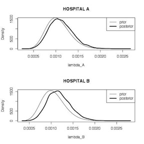
Hospital Mortality Comparison
Conjugate Analysis of Normally Distributed Data
It may appear a bit odd to place a discussion of the normal distribution after binomial and Poisson, but I have my reasons. First, I think most epidemiologists will get the most immediate use out of the martial about proportions and counts. Second, despite it’s fundamental role in statistics, the normal distribution is when we start reaching the limits of simple conjugate analyses. This may be a bit disconcerting, but not to worry. We will soon use the normal distribution as a springboard to computational approaches to more complex and realistic data problems. For now, though, let’s walk through a simple conjugate analysis of normally distributed data.
When you have normally distributed data (likelihood \(x \sim Nl(\theta, \sigma^2)\)), and a normally distributed prior (\(\theta \sim Nl(\mu, \sigma^2)\)), the posterior is basically a weighted average of the prior mean and the parameter estimate of the data mean, weighted by their precisions. We will have to estimate an “implicit” sample size for the prior, \(n_0\), using the s.d. of the prior. You will find (and this is generally the case in Bayesian analyses) that as the sample size of the data increases, the posterior gets “swamped” by the data, and is essentially the MLE estimate.
Example: THM Concentrations
Local public health agencies test water samples for trihalomethanes (THMs) in every supply zone a couple of times each year. We want to estimate the average concentration in a particular zone \(z\) based on two measurements (\(x_{z1}\) and \(x_{z2}\) ) with mean \(x_{z \mu} = 130\), which has \(\sigma=5\). What is the best estimate of the mean concentration (\(\theta\))?
The MLE or frequentist approach would use the mean concentration, 130, as the point estimate for \(\theta\) with a s.e. of \(\sigma / \sqrt{n} = 5 / \sqrt{2} = 3.5\) for a 95% CI of 130 \(\pm\) 1.96 * 3.5 = 123.1, 136.9.
A Bayesian approach could use information from previous years to inform the analyses. Say data from previous years indicated a THM concentration of 120 with a s.d. = 10. This suggests a prior of \(\theta \sim Nl(120,10^2)\) We solve for the “implicit” sample size for the prior as \(s.d.= \sigma / \sqrt{n_0}\), \(n_0 = (\sigma / 10)^2 = .25\), or equivalent to about \(\frac{1}{4}\) of an observation. The prior can be written as \(\theta \sim Nl(120, \sigma^2/.25)\), and the posterior is:
\[ p(\theta | x) = Nl(0.25*120 + 2*130 / 0.25 + 2, 52/0.25+2) \\ = = Nl( 128.9, 3.332) \]
and a 95% CI for \(\theta\) of 122.4, 135.4
In this figure, we can see the relation of the prior, the likelihood and posterior. The posterior is basically a combination of data and prior knowledge; the interval tends to be narrower than the likelihood
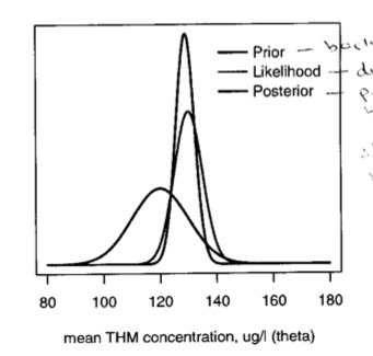
We can, as we did with the binomial and Poisson examples, make predictions based on this posterior. The predictive distribution is centered around the posterior mean with variance equal to the sum of the posterior variance and the sample variance, \(\sim Nl(\mu, \sigma^2_n + \sigma^2)\) Continuing the example, suppose the water company will be fined if the THM level exceeds 145. We can calculate the probability that a future sample will exceed 145 as the posterior predictive distribution \(Nl(128.9, 3.332 + 5^2)\) = \(Nl(128.9, 36.1)\), with the tail probability of a value greater than 145 = 0.004
Probability Distributions Used in Bayesian Analysis
As you can see, one of the hallmarks of Bayesian analysis is the explicit use of probability distributions to describe the behavior of both variables and the parameters that govern those variables. Bayesians tend to spend a lot of time thinking about which distributions most closely fit the behavior they are trying to describe. In addition to being more comfortable with probability theory in general, you will need to become more familiar with some probability distributions with which you may only have passing acquaintance. 12
Bayesian analyses tend toward flexible distributions, i.e. the form changes based on parameters. Some important ones include:
The Beta Distribution
\[ \sim Beta(\alpha,\beta)\\ \mu=\frac{\alpha}{\alpha+\beta}\\ \sigma^2=\frac{\alpha \beta}{(\alpha \beta)^2 (\alpha + \beta) + 1} \]
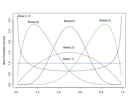
The Beta Distribution
The beta distribution returns values between 0 and 1, os is often used to model proportions and probabilities. \(\alpha\) is the prior number of successes, \(\beta\) is the prior number of failures. As you can see from the figure, the beta distribution is quite flexible in its form, which contributes to its popularity in Bayesian analyses (It is also conjugate to the binomial distribution, a concept we’ll discuss shortly). For a flat prior, set both \(\alpha\) and \(\beta\) equal to 1. Setting both \(\alpha > 0\) and \(\beta > 0\) ensures a proper distribution that can be integrated. For a unimodal distribution, set both \(\alpha > 1\) and \(\beta > 1\). As \(\alpha, \)$, the closer the distribution approaches normality.
The BUGS syntax for the beta distribution is
1 | dbeta(alpha, beta) |
The Gamma Distribution
\[ \sim \Gamma(\alpha, \beta),\\ \mu=\frac{\alpha}{\beta} \\ \sigma^2=\frac{\alpha}{\beta^2} \]
Where, \(\alpha\) is the “shape” parameter and \(\beta\) is the “scale” parameter.
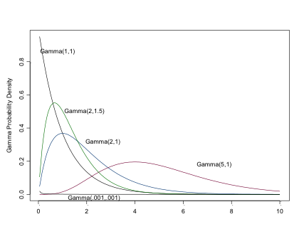
The Gamma Distribution
Setting \(\alpha=1\) results is an exponential distribution (\(\mu=1/\beta\)). \(\sim \Gamma(\alpha/2, 1/2)\) is \(\chi^2\) with \(\alpha\) d.f.
Like the exponential distribution (of which it is a more general case), you can use this very flexible distribution for positive continuous variables, e.g. counts or time to events. (You can see why the Gamma distribution may be of considerable interest to epidemiologists). The Gamma distribution is often seen as a prior for a Normal precision parameter, and prior for Beta parameters.
In BUGS, it is specified
1 | dgamma(alpha, beta) |
You can obtain a flat prior by setting \(\alpha\) and \(\beta\) to be small, eg dgamma(.001,.001)
The Normal Distribution
\[ \sim Nl(\mu, \sigma^2) \]
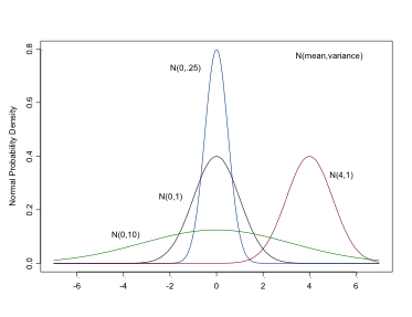
The Normal Distribution
This is the distribution with which you are likely most familiar. It is used for both likelihoods and priors for continuous variables or parameters. In BUGS it is specified as:
1 | dnorm(mean, precision) |
Note that in BUGS, probability distributions are specified in terms of their precisions, \(1/\sigma^2\). So for a flat prior, which would have a very large variance, you would instead specify a very small precision, e.g. dnorm(0,.0001) , or dnorm(0,1.0E-4).
You can restrict a prior to positive values (for example for a standard deviation), by using the half-normal prior available in BUGS:
1 | dnorm(0,1.0E-4)I(0,) |
BUGS also accommodates the other two most commonly used distributions in epidemiology, the binomial and the Poisson.
1 2 | dbin(p,n) dpois(lambda) |
The Uniform Distribution
\[ \sim Unif(a,b), \\ \mu = \frac{(a+b)}{2}, \\ \sigma^2 = \frac{(b-a)^2}{12} \]
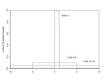
The Uniform Distribution
Uniform distributions are useful for parameters that can only take values on a specific interval (a,b), e.g. standard deviations, or for proportion parameters on the interval (0,1). In BUGS it is specified:
1 | dunif(a,b) |
For a “flat prior”, set the range to be large, e.g. dunif(-100,100) or dunif(0,100) for positive parameters
The Exponential Distribution
\[ \sim Exp(\lambda),\\ mu=1/\lambda,\\ \sigma^2=1/\lambda^2 \]
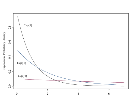
The Exponential Distribution
The exponential distribution can be used to model the likelihood for positive continuous variables, especially time to events, or as a prior for Beta-distributed parameters. For a “flat prior”, set lambda to be small, eg dexp(.01)
The Dirichlet Distribution
\[ \sim Dirichlet(\alpha_1, ... \alpha_k) \]
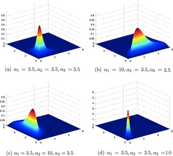
The Dirichlet Distribution
Where \(\alpha_i\) is a vector of the prior number of outcomes of type i, is used for multinomial proportions or probabilities (i.e, take values between 0 and 1). It is an extension of the Beta distribution for several probability parameters that must sum to 1. For a flat prior, se alpha as a vector of 1’s: c(1,1,….,1).
The BUGS syntax is
1 | ddirch(alpha[]) |
In classical statistics, parameters are somewhat Aristotelian. We believe they exist in some perfect state, but we may never directly observe them, only the shadows they cast on our samples.↩
Don’t worry if your calculus is a little rusty. The last time I took a derivative or an integral most folks still had rotary phones. A basic understanding, but not much more, is all that is required for the practical application of Bayesian statistics.↩
For a fuller description of Bayes Theorem see this document↩
There is a more intuitive way of making this calculation. The probability of someone having a positive test given that they have the disease is the number of positive tests over the number of people with disease. In this example, that is 498/508. In statistical terms, this approach uses the marginal probability of disease to simplify the calculations. We will explore and take advantage of marginal probabilities as a simplifying strategy for future, more complex situations.↩
The models in this section come from Dr. Shane Jensen’s excellent short course on Bayesian Data Analysis given through Statistical Horizons. I highly recommend it.↩
I suppose you could, if you really tried, find out how many flights there were each year…↩
You may be asking yourself (as I did when I first encountered this material) why we just didn’t use a binomial prior for the binomial likelihood, or a Poisson prior for a Poisson likelihood. The short answer is that they just don’t work. The longer answer has to do with what results when you multiply one distribution by another (binomialbinomial and PoissonPoisson are apparently particularly ugly) as well as issues with dependence of parameters that arise.↩
The factorial notation ! and stands for \(n x n-1 x n-2 x ... x n- ( )\))↩
This neat analytic approach results in a so-called “closed” result. A closed result refers to the fact that the distributions play nicely together can be integrated to a single solution, which in the case-of all probability distributions sums to one.↩
Note that the \(\binom{n}{k}\) term drops out of the calculations because it is simply a normalizing constant and isn’t necessary for the calculation of ratios.↩
Because of the larger number of observations, we are presenting the likelihood on the log scale.↩
Despite the availability and popularity of some of these more exotic probability distributions, some very smart folks (like David Spiegelhalter at Cambridge) believe the majority of analyses can readily be accomplished with the 4 most common distributions: binomial, normal, poisson and uniform.↩