The Recipe

Difference between two groups on continuous measurement

$\Delta = y_0 - y_1$ - Difference
$\mu_{\Delta} = 0$ - No mean difference (Curve on the left)
$\mu_{\Delta} = \delta$ - Appreciable mean difference (Curve on the right)
$\sigma^2$ - Variances equal
$se_{\Delta} = \sigma * \sqrt{\frac{2}{n}}$ - The relationship between the standard error of the differences in means and the standard deviation allows us to set up calculations for the sample size, $n$.
- $\sigma \sqrt{\frac{2}{n}}$ derives from the s.e. for difference means with equal variances

The Critical Value

Difference between two groups on continuous measurement

where the upper value of $\alpha$ on the null curve meets and the value for $\beta$ on the alternative curve
- point at which you accept or reject your null hypothesis \[ 0 + z_{1-\alpha/2} * \sigma \sqrt{\frac{2}{n}} = \delta - z_{1-\beta} * \sigma \sqrt{\frac{2}{n}} \]
Solve for $n$ \[ n_{group}=\frac{2(z_{1-\alpha/2} + z_{1-\beta})^2}{(\frac{\mu_1 - \mu_2}{\sigma})^2} \]

“Classic” Formulation

Difference between two groups on continuous measurement

Conditional probabilities
type I error or $\alpha$ = Pr[+ result | - difference], ie. false positive
- the black-shaded 0.05/2 tails on the null hypothesis
type II error or $\beta$ = Pr[- result | + difference], i.e. false negative
- the hatched 0.2 left-handed tail on the alternative hypothesis
power or $1 - \beta$ = Pr[+ result | + difference], i.e. true positive
- the area to the right of $\beta$ on the alternative hypothesis

More Bang for your Buck

Difference between two groups on continuous measurement

Increase AUC to the right of the critical value
Measure your outcome more precisely
- “shrinks” curves towards means
study a greater effect size
- increases difference between $\mu_{\Delta} = 0$ and $\mu_{\Delta} = \delta$, separates the curves more

CONTINUOUS MEASUREMENTS

Lehr’s Equation (Difference Between Two Means)

Substitute the usual values of 1.96 for $\alpha$ and 0.84 for $\beta$
Recognize denominator as the square of the standardized difference ($\Delta ^2$) \[ n_{group}=\frac{2(1.96 + 0.84)^2}{(\Delta)^2} \\ n_{group}=\frac{16}{(\Delta)^2} \]
10-point difference in IQ between two groups (mean population IQ of 100, and a standard deviation of 20): \[ n_{group}=\frac{16}{((100-90)/20)^2} \\ n_{group}=\frac{16}{(.5)^2} \]
total sample size of 128.
function in R

nMeans<-function(x0, x1, sd){
    d<-(x1-x0)/sd           
    n<-16/d^2
    n
    }
nMeans(100,90,20)

Evaluate range of values

Possible mean difference between the two groups anywhere between 2 and 10 IQ points

1
2
3

unexp<-100
exp<-seq(88,98,2)
nMeans(unexp, exp, 20)

Standard deviation somewhere between 10 and 20 IQ points

1 2	`dev<-seq(10,20,2) nMeans(100, 90, dev)`

Combination of difference and variation

for(i in seq(10,20,2)){
    size<-nMeans(unexp,exp, i)
    print(size)
}

Detectible Difference Between Two Means

Rearrange Lehr’s equation to solve for the detectible standardized difference between two populations: \[ n_{group}=\frac{16}{(\Delta)^2} \\ (\Delta)^2 = \frac{16}{n_{group}} \\ \Delta = \frac{4}{\sqrt{n_{group}}} \\ \]
unstandardized difference \[ \delta = \frac{4 \sigma}{\sqrt{n_{group}}} \]

nDD<-function(sd, n){  
    dd<-4*sd/(sqrt(n))
    dd
    }

Detectible difference in mean IQ with a sample size of 50

1	`nDD(20,50)`

about 12 IQ points.

Percentage Change in Means

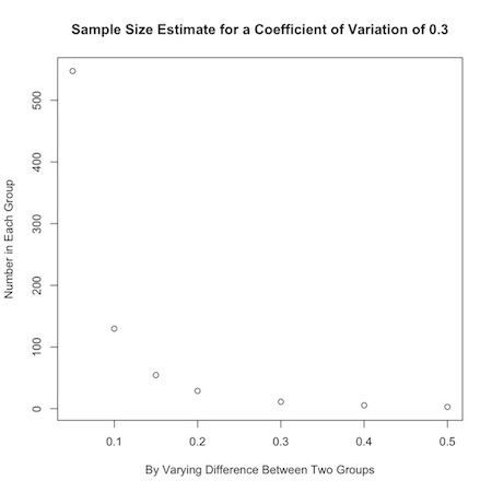
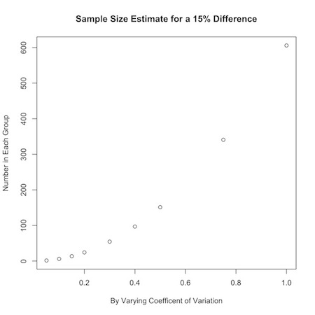
- \[ n_{group}=\frac{16(c.v.)^2}{(ln(\mu_0)-ln(\mu_1))^2} \\ n_{group}=\frac{16(c.v.)^2}{(ln(r.m.))^2} \]
where,
- $c.v. = \sigma / \mu$
- r.m - percentage change translated into ratio of means \[ = \frac{\mu_0 - \mu_1}{\mu_0} = 1 - \frac{\mu_1}{\mu_0} \]
e.g.20% difference between two groups in data with about 30% variability.
- 20% change translates to a ratio of means of $1-.20=.80$.
  \[ n_{group}=\frac{16(.3)^2}{(ln(.8))^2} = 29 \]
R function

nPC<-function(cv, pc){
    x<-16*(cv)^2/((log((1-pc)))^2)
    print(x)
}

15% change from one group to another, but uncertain about how the data varies

a<-c(.05,.10,.15,.20,.30,.40,.50,.75,1)
nPC(a,.15)

plot(a,nPC(a,.15),  ylab="Number in Each Group", 
xlab="By Varying Coefficent of Variation", 
main="Sample Size Estimate for a 15% Difference")

Or look at how desired effect size changes sample calculations

1
2
3

plot(b, nPC(.3,b), ylab="Number in Each Group", 
xlab="By Varying Difference Between Two Groups", 
main="Sample Size Estimate for a Coefficient of Variation of 0.3")

no idea about c.v?
- 0.35 is a handy substitute for many biological systems

POISSON DISTRIBUTED OR COUNT DATA

The square root of poisson-distributed data is approximately normally distributed,

- \[ y_i \sim Pois (\lambda) \\ \sqrt{y_i} \sim Nl(\sqrt{\lambda}, 0.25) \]
apply Lehr’s equation by taking the square root \[ n_{group}=\frac{4}{(\sqrt{\lambda_1}-\sqrt{\lambda_2})^2} \]
mean count of health outcome = 36 per unit of observation (e.g. person-year)
want to demonstrate decrease to 30 per unit of observation in a comparison population
$n_{group}=\frac{4}{(\sqrt{30}-\sqrt{36})^2} = 15$ units of observations in each group.
mean counts per unit time (or volume )
- mean is $T * \lambda$
- $n_{group}=\frac{4}{T * (\sqrt{\lambda_1}-\sqrt{\lambda_2})^2}$
high background rates of disease, $\lambda *$
- add background rate to the individual means
- $n_{group}=\frac{4}{(\sqrt{\lambda_1 + \lambda *}-\sqrt{\lambda_2 + \lambda *})^2}$
two Poisson sets data with means $\mu_1=1$ and $\mu_2=2$
- $n_{group}=\frac{4}{(\sqrt{2}-\sqrt{1})^2} = 25$ observations in each group.
- background population rate of 1.5,
- $n_{group}=\frac{4}{(\sqrt{3.5}-\sqrt{2.5})^2} = 50$
rate above background for significant result ($\Delta_{\lambda}$)
- set $\lambda_1$ to 0 and $_2$ to $\Delta_{\lambda}$
- $\Delta_{\lambda} = 4 \sqrt{\lambda *}$
need 4 times the square root of the background rate more outcomes
- e.g. usually 50,000 deaths in a population
- need $4 \sqrt{50000} = 895$ more deaths to demonstrate the effect of some event

R functions for Poisson-distributed data

 # count data, x= population mean
nPois<-function(x0,x1){        
    n<-4/(sqrt(x0)-sqrt(x1))^2    
    n    
    }
nPois(1,2)

 #takes background rate x into account
nbrPois<-function(x,x0,x1){        
    n<-4/(sqrt(x+x0)-sqrt(x+x1))^2    
    n    
    }
nbrPois(1.5,1,2)


 # n beyond background rate needed
nbbrPois<-function(x){             
    n<-4*sqrt(x)
    n
    }
nbbrPois(50000)

Upper Bound for Count Data when No Events Have Occurred (Rule Of 3)

Given no events or outcomes in a series of $n$ trials, the 95% upper bound of the rate of occurrence \[ \frac{3}{n} \]
E.g. 20 surgeries, not bad outcomes
- $3/20=0.15$ or 15% chance of an adverse event
Derives from sum of independent Poison variables also Poisson
- $n$ trials of $Pois(\lambda)$ process is $Pois(n \lambda)$
- probability of at least one non-zero trial is 1 minus the probability that all the trials are zero
- $Pr[some_{1}] = Pr[1-\forall_{0}]$
Set probability to statistical significance *$1-0.95 = 0.05 = Pr[\Sigma y_1 = 0] = e^{n \lambda}$ *$n \lambda = -ln(0.05) = 2.996$ *$\lambda \approx 3/n$

Relative Risks and Odds Ratios

(Again) based on Poisson distribution
$n_{group} = \frac{4}{\frac{c}{c+d} (\sqrt{RR}-1)^2}$
reasonably accurate for prevalences under 20%
E.g. to detect RR at least 3 in study of disease with prevalence of 1% in unexposed
$n_{group} = \frac{4}{0.01 (\sqrt{3}-1)^2} = 746.4$
increasing prevalence, decreases required sample size
- can increase period of observation

number of outcomes needed to detect a relative risk

rearrange the formula
$c = n_{group} * \frac{c}{c+d} = \frac{4}{(\sqrt{RR}-1)^2}$
E.g. for RR at least 3
$4/ (\sqrt{3}-1)^2 \approx 8$ outcomes in unexposed
$3 * 8 = 24$ outcomes in the exposed
just the flip side of the previous formula
- rates of 1/100 in exposed and 3/100 in unexposed require 747 people in each group
number of outcomes that crucial, not necessarily number of exposed and unexposed.

Log-Based Formulas

for RR *$n_{group} = \frac{8(RR+1)/RR}{\frac{c}{c+d} (ln(RR))^2}$
for OR
- $n_{group} = \frac{8 \sigma^2_{ln(OR)}}{(ln(OR))^2}$
where, for prevalence $p_0$ unexposed and $p_1$ exposed *$\sigma^2_{ln(OR)} = \frac{1}{p_0} + \frac{1}{1-p_0} +\frac{1}{p_1} +\frac{1}{1-p_1}$
- ln(OR) = $ln(\frac{(p_1)(1-p_0)}{(1-p_1)(p_0)})$
E.g. unexposed prevalence 1%, to achieve RR 3
- $n_{group} = \frac{8(4)/3}{0.01 (ln(3))^2} \approx 884$
for OR 3
- $n_{group} = 8 * (\frac{1}{.01} + \frac{1}{.99} +\frac{1}{.03} +\frac{1}{.97}) / ln(\frac{(.03)(.99)}{.97) (.01)})^2 \approx 865$
log-based formulae more conservative than Poisson-based
- Sample size calculations are not prescriptive

BINOMIAL DATA OR PROPORTIONS

average the two proportions to adapt Lehr’s equation
- $\bar{p} = (p_0 + p_1)/2$
- $n_{group}=\frac{16 \bar{p} \bar{q}}{(p_0 - p_1)^2}$
E.g. outcome 30% in untreated population
want to demonstrate treatment decreases to 10%.
- $\bar{p} = (.3 + .1)/2 = .2$ and $\bar{q} = 1-.2 = .8$, and $n_{group}=\frac{16 * .2 * .8}{(.3 - .1)^2} = 64$
most conservative (maximum) variance estimate
- $p_0=.5$
$\bar{p} = (.5 + .5)/2 = .5$
- numerator of sample size calculation $16 * .5 *.5 = 4$:
- $n_{group}=\frac{4}{(p_0 - p_1)^2}$
E.g. $n_{group}=\frac{4}{(.3 - .1)^2} = 100$
conservative approximation only valid where sample size each group between 10 and 100

The Rule of 50

For rare, discrete outcomes, you need at least 50 events in a control group, and an equal number in a treatment group, to detect a halving of risk.
E.g. risk of MI 8% over 5 years
want to demonstrate drug reduces risk to 4%
need enough patients to have 50 MI’s in each arm of the study
- 50 / 0.08 = 625 patients in each group, or 1,250 subjects in total
- conservative ballpark, actual calculations return value of 553 each group.
derivation of rule of 50
- from the sample size calculation for a binomial sample
- $n_{group} = \frac{(z_{1- \alpha / 2} \sqrt{\bar{pq}(1+\frac{1}{k})} + z_{1- \beta} \sqrt{\frac{p_1 q_1}{p_2 q_2}})^2}{\Delta ^2}$
event is rare, so $p_1 \approx p_2$ and is very small, and $q_1 \approx q_2 \approx 1$
- $n_{group} = \frac{(z_{1- \alpha / 2} \sqrt{\bar{p}(1+\frac{1}{k})} + z_{1- \beta} \sqrt{\frac{p_1}{p_2}})^2}{\Delta ^2}$
for 50% decline group 1 to group 2, $p_2 = .5p_1$ and $\bar{p} = .75p_1$.
for equal sample sizes (k=1), and the standard alpha an beta, formula simplifies
- $n_{group} = \frac{(1.96 \sqrt{1.5p_1} + 0.84 \sqrt{1.5p_1})^2}{(0.5p_1) ^2}$
solving for $n_{group}p_1$ results in 47
- round up to 50.

MORE RULES OF THUMB FROM GERALD VAN BELLE

A quick estimate of the standard deviation is $s = \frac{Range}{\sqrt{n}}$
Confidence intervals can overlap as much as 29% and still be statistically significantly different
In a logistic regression, aim for about 10 outcomes for every parameter in the model
Little to be gained, beyond 4 or 5 controls per case
Surprisingly little optimization in overall costs with unequal sample sizes even the costs for one population are appreciably greater than the other,

A (Bayesian) Twist to Lehr’s Equation

power calculation are a guide, not a requirement
should be run over range of possible effect sizes and standard deviations
logical step to run over a distribution
incorporating uncertainty is inherently Bayesian
E.g. 10 point difference in IQ two groups, sd=20
estimate from Lehr’s formula 64 each group
say believe estimate for sd has its own distribution
- $\mu=20$ and $\sigma^2=1$
also believe estimate for difference has its own distribution
- $\mu=10$ and $\sigma^2=1$
redefine basic Lehr’s formula R function in terms of difference and standard deviation.

nMeans.vary<-function(diff, sd){   
    d<-diff/sd              
    n<-16/d^2
    n
    }

sample from a distribution
- because negative sd makes no sense, use the truncated normal distribution

install.packages("truncnorm")
library(truncnorm)

sd.r<-rtruncnorm(n=1000, a=0, mean=20, sd=1)
diff.r<-rtruncnorm(n=1000, a=0, mean=10, sd=1)

n1<-nMeans.vary(diff.r,sd.r)
summary(n1)
plot(density(n1))

can achieve same power under the same conditions with a few as 30 or as many as 160 observations in each group.
alternatively, look at how power varies for the point estimate of 64 observations in each group
solve for power given a sample size $n$, a difference between two groups of $\theta$ and a standard deviation of $\sigma$:
Power = $\phi (\sqrt{\frac{n \theta ^2}{2 \sigma ^2}}-1.96)$


p1<-sqrt(64/2) * diff.r/sd.r -1.96

summary(pnorm(p1))
plot(density(pnorm(p1)))

power of study with 64 observations in each group can be as low as 42% or has high as 98%.

“ADAPTIVE” BAYESIAN DESIGNS

traditional approach

disease 25% prevalence
want to demonstrate decrease to 10%
- efficacy 40% (.1/.25)
use Lehr’s equation
$n_{group}=\frac{16 \bar{p} \bar{q}}{(p_0 - p_1)^2}$

nBin<-function(p0,p1){
    p<-(p0+p1)/2
    n<-16*p*(1-p)/(p0-p1)^2
    n   
    } 
nBin(.25,.1)

take limited resources into account

only enough money to enroll 20 patients
reframe the question: What is the probability that (say) 15 of the twenty will respond?
again, believe about 40% efficacy
but now, add belief efficacy ranges between 20% to 60% with sd of 10%
use this info to define a Beta distribution to use as a prior in a binomial simulation
define parameters for Beta prior from mean and variance

estBetaParams <- function(mu, var) {
  alpha <- ((1 - mu) / var - 1 / mu) * mu ^ 2
  beta <- alpha * (1 / mu - 1)
  return(params = list(alpha = alpha, beta = beta))
}

estBetaParams(.4,(.1)^2)

use the Beta distribution to define a binomial simulation to answer question

N=1000
theta<-rbeta(N,9.2,13.8)
x<-rbinom(N,20, theta)
y<-0
accept<-ifelse(x>14.5, y+1, y+0)
prob<-sum(accept)/N
prob
library(coda)
densityplot(accept)

power is simply the proportion of simulations that meet or exceed the criteria of being greater than or equal to 15
- here about a 2% probability that a study of 20 patients will show efficacy in 15 people.

take what’s known into account

find study that demonstrates efficacy in 15 of 20 patients
incorporate information by updating the Beta prior
use “conjugacy”
- $Beta$ priors and $Binomial$ likelihoods
if prior is \[ \theta \sim Beta(a,b) \]
and the likelihood is \[ X| \theta \sim Bin (N, \theta) \]
then the posterior is \[ \theta | X \sim Beta (X+a, N-X+b) \]
new prior for $\theta$ in planned study is $Beta(15+9.2, 20-15+13.8)$
combines Binomial ${20 \choose 15} p^{15}q^{20-15}$ likelihood of external data with the $Beta(9.2, 13.8)$,

N=1000
theta<-rbeta(N,24.2,18.8)
x<-rbinom(N,20, theta)
y<-0
accept<-ifelse(x>14.5, y+1, y+0)
prob<-sum(accept)/N
prob

probability of demonstrating target efficacy has gone up
- though clearly not as much as we want

from updating to adapting

do the study and find 14 of 20 patients respond
make a “decision rule”: if see 25 responses in next 40 patients will continue drug development
how likely is that to be?
again a matter of updating the prior and running the simulation
updated prior for $\theta$ is $Beta(14+24.2,20-14+18.8)$
probability of 25 or more successes in an additional 40 trials is about 38%
- judgement on whether that is a good “rule”

N=1000
theta<-rbeta(N,38.2,24.8)
x<-rbinom(N,40, theta)
y<-0
accept<-ifelse(x>25, y+1, y+0)
prob<-sum(accept)/N
prob

learn from accumulating evidence
designs adapt
decisions based on predictive probabilities
- early stopping, re-estimation of sample sizes, weighting the randomization process
best suited to settings where patients enrolled quickly, responses ascertained quickly, costs high, uncertainty about effect
requires additional, sometimes complex initial planning, considerable flexibility, regulatory approvals, concerns may increase type I error because multiple analyses, concerns may introduce bias because know results or through patient selection

Bayesian Sample Sizes

where are the sample size calculations?
rather than run calculations for a set sample size (as above) replace with a vector of values

Nrep<-1000
s<-40:100
theta<-rbeta(Nrep,38.2,24.8)
y<-0

results<-matrix(0, nrow=length(s), ncol=1)
for(i in 1:length(s)){
x<-rbinom(Nrep,s[i], theta) 
accept<-ifelse(x>25, y+1, y+0)
prob[i]<-sum(accept)/Nrep
results[i,]<-prob[i]
}

tab<-cbind(s, results)

tab

hit the usual 80% threshold with a sample of about 49.

weighting evidence

till now have applied equal weighting to prior study or evidence
can downweight previous study data with weight $0 \le w \le 1$l
- likelihood, $Beta(a*w, b*w)$
- each previous patient info worth fraction $w$ of new patient info
E.g. not very confident of the evidence from the literature
downweight it by 50%
take $Beta(24.2,18.8)$ prior and multiply through by .5
- $Beta(24.2*.5,18.8*.5)$
then update with the evidence from the trial
- $Beta(14+12.2, 20-14+14.4)$

Nrep<-1000
s<-40:100
theta<-rbeta(Nrep,26.2,20.4)
y<-0

results<-matrix(0, nrow=length(s), ncol=1)
for(i in 1:length(s)){
x<-rbinom(Nrep,s[i], theta) 
accept<-ifelse(x>25, y+1, y+0)
prob[i]<-sum(accept)/Nrep
results[i,]<-prob[i]
}

tab<-cbind(s, results)

tab

now don’t hit 80% power until a sample size of about 54.
can shift or manipulate the prior
- keep overall sample size same
- increase or decrease the number of successes that go the beta-binomial conjugate calculation
E.g. take the $Beta(14+24.2,20-14+18.8)$ prior and shift 7 of the successes to failures as $Beta(7+24.2,20-7+18.8)$

Nrep<-1000
s<-40:100
theta<-rbeta(Nrep,31.2,31.8)
y<-0

results<-matrix(0, nrow=length(s), ncol=1)
for(i in 1:length(s)){
x<-rbinom(Nrep,s[i], theta) 
accept<-ifelse(x>25, y+1, y+0)
prob[i]<-sum(accept)/Nrep
results[i,]<-prob[i]
}

tab<-cbind(s, results)

tab

now have to increase the sample size to 61 to achieve the same power.

Power Tools for Epidemiologists

Acknowledgements

COOKING A SAMPLE SIZE

Two Key Ingredients

The Recipe

The Critical Value

“Classic” Formulation

More Bang for your Buck

CONTINUOUS MEASUREMENTS

Lehr’s Equation (Difference Between Two Means)

Evaluate range of values

Detectible Difference Between Two Means

Percentage Change in Means

Or look at how desired effect size changes sample calculations

POISSON DISTRIBUTED OR COUNT DATA

The square root of poisson-distributed data is approximately normally distributed,

R functions for Poisson-distributed data

Upper Bound for Count Data when No Events Have Occurred (Rule Of 3)

Relative Risks and Odds Ratios

number of outcomes needed to detect a relative risk

Log-Based Formulas

BINOMIAL DATA OR PROPORTIONS

The Rule of 50

MORE RULES OF THUMB FROM GERALD VAN BELLE

BAYESIAN APPROACH

A (Bayesian) Twist to Lehr’s Equation

“ADAPTIVE” BAYESIAN DESIGNS

traditional approach

take limited resources into account

take what’s known into account

from updating to adapting

Bayesian Sample Sizes

weighting evidence