A Brief Introduction to Spatial Analysis in R

See these more thorough overviews:

Let’s wade right in…

first steps

plotting the meuse data

1
2
3
plot(meuse)
plot(meuse$x, meuse$y)
plot(meuse$y, meuse$x)

SpatialPointsDataFrame object

1
2
3
coordinates(meuse) <- ~x+y
str(meuse)
plot(meuse)

categorize and plot flood frequencies

1
2
3
4
5
meuse$ffreq <- as.numeric(meuse$ffreq)
plot(meuse, col = meuse$ffreq, pch = 19)
labs <- c("annual", "every 2-5 years", "> 5 years")
cols <- 1:nlevels(meuse$ffreq)
legend("topleft", legend = labs, col = cols, pch = 19, bty = "n")

working with spatial objects

1
2
spplot(meuse, "zinc")
bubble(meuse, "lead")

coordinate reference systems

1
proj4string(meuse) <- CRS("+init=epsg:28992")

Why map?

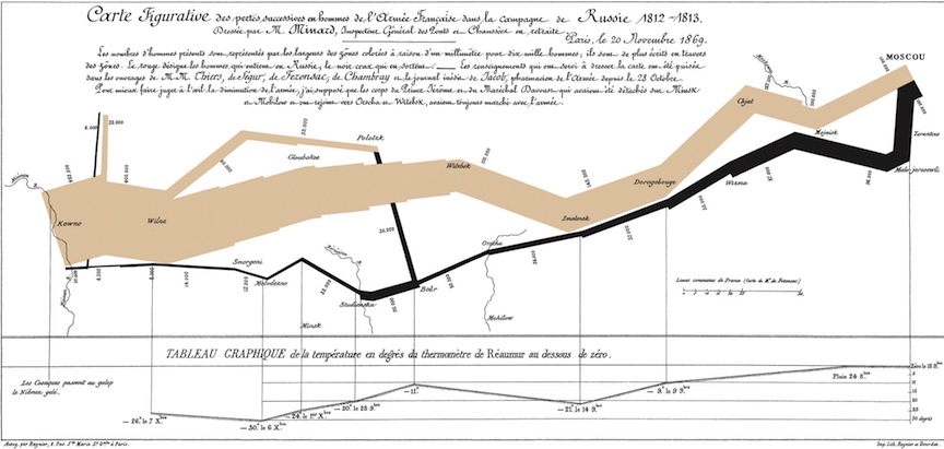
The greatest map?

Minard’s Map of Napolean’s Russian Campaign of 1812

Minard’s Map of Napolean’s Russian Campaign of 1812

Minard’s Map Illustrates 6 principals (6 C’s) of analytic design and mapping (from Tufte)

Spatial Analysis

R and Spatial Analysis

R spatial data

R spatial packages

3 Basic Applications

Areal Data: Suicide Mortality in 32 London Boroughs 1989-1993

1
2
3
4
5
6
7
8
9
10
11
12
13
14
15
16
library(maptools)
library(spdep)

london<-readShapePoly("~ download ~ /LDNSuicides")
plot(london) # NB: no CRS
class(london)
names(london)
london$NAME

obs=c(75,145,99,168,152,173,152,169,130,117,124,119,134,90,
    98,89,128,145,130,69,246,166,95,135,98,97,202,75,100,
    100,153,194) # observerd number suicides each london borough
exp=c(80.7,169.8,123.2,139.5,169.1,107.2,179.8,160.4,147.5,
    116.8,102.8,91.8,119.6,114.8,131.1,136.1,116.6,98.5,
    88.8,79.8,144.9,134.7,98.9,118.6,130.6,96.1,127.1,97.7,
    88.5,121.4,156.8,114) # expected number suicides each london borough
1
2
NAME<- sort(london$NAME)
suicide.dat <- data.frame(NAME=NAME, obs=obs, exp=exp)
1
2
3
4
suicide.dat$SMR<-suicide.dat$obs/suicide.dat$exp

library(DCluster)
suicide.dat$smooth <- empbaysmooth(suicide.dat$obs,suicide.dat$exp)$smthrr

map the results

1
2
3
data.london<-attr(london,"data")
order<-match(data.london$NAME,suicide.dat$NAME)
suicide.dat<-suicide.dat[order,]
1
2
3
4
5
6
cuts<- c(0.6, 0.9, 1.0, 1.1,  1.8)
suicide.dat$SMR.cut<-cut(suicide.dat$SMR,breaks=cuts,include.lowest=TRUE)
suicide.dat$smooth.cut<-cut(suicide.dat$smooth,breaks=cuts,include.lowest=TRUE)
attr(london,"data")<-merge(data.london,suicide.dat,by="NAME")

spplot(london, c("SMR.cut", "smooth.cut"),col.regions=gray(3.5:0.5/4),main="")

Point Process Data: Broad Street Pump Cholera Outbreak

load packages, read data (with rgdal), plot

1
2
3
4
5
6
7
8
library(spatstat)
library(rgdal)

cholera<-readOGR(" ~ download ~ /Cholera_Deaths.shp", "Cholera_Deaths")
pumps<-readOGR("~ download ~ /Pumps.shp", "Pumps")

plot(cholera, pch=16)
plot(pumps, add=T, col="red", pch=10, cex=3)

plot with background image

1
2
3
4
5
6
bkgrnd<-readGDAL(" ~ download ~ /Cholera_Deaths/SnowMap.jpg")

plot(cholera, pch=16)
image(bkgrnd,col = grey(1:99/100), add=T)
plot(cholera, pch=16, add=T, col="red")
plot(pumps, add=T, col="blue", pch=10, cex=3)

plot the point process with spatstat

1
2
3
4
5
6
7
8
9
10
11
12
cholera.point<-as.ppp(cholera)
summary(cholera.point)
plot(cholera.point)

plot(density(cholera.point,20))
plot(density(cholera.point,30))
plot(pumps, add=T, col="red", pch=10, cex=3)


persp(density(cholera.point,30))
persp(density(cholera.point,30), theta=90)
persp(density(cholera.point,30), theta=180)

Riply’s K statistic

1
2
cholera.k<-Kest(cholera.point)
plot(cholera.k)

Spatial Interpolation