A Brief Introduction to Spatial Analysis in R

See these more thorough overviews:

• Roger Bivand - very highly recommended, and the basis for much of my material
• notes and tutorial
• chapter on spatial mapping of overdose deaths
• course exercise

Let’s wade right in…

first steps

• install and load sp and maps
• load the meuse data set
• examine the structure of meuse
  • dataframe, 155 observations, 14 variables
  • x and y are map coordinates

plotting the meuse data

1
2
3

plot(meuse)
plot(meuse$x, meuse$y)
plot(meuse$y, meuse$x)

SpatialPointsDataFrame object

• spatially-referenced points with attribute data
• sp:coordinates() will convert R dataframe to SpatialPointsDataFrame

1
2
3

coordinates(meuse) <- ~x+y
str(meuse)
plot(meuse)

categorize and plot flood frequencies

1
2
3
4
5

meuse$ffreq <- as.numeric(meuse$ffreq)
plot(meuse, col = meuse$ffreq, pch = 19)
labs <- c("annual", "every 2-5 years", "> 5 years")
cols <- 1:nlevels(meuse$ffreq)
legend("topleft", legend = labs, col = cols, pch = 19, bty = "n")

working with spatial objects

• Spatial objects are S4 objects
• note in str() output, uses the @ convention
• e.g. names(meuse@data)
• some special spatial tools, e.g select.spatial() to identify points
• select.spatial(meuse)
  • click three points to surround (don’t have to completely surround)
  • R click to return point data
• generic plot() return spatially-referenced results, e.g plot()
• …but special spatial plots are available

1
2

spplot(meuse, "zinc")
bubble(meuse, "lead")

coordinate reference systems

• definitions for the location of a point on the earth
• reference ellipsoid - defines shape of the earth
• datum - reference point(s) on earth’s surface
• unit of measurment, e.g. meters, miles
• projection - how spherical earth projected onto 2 dimensions
  • equirectangular
  • cylindrical or Mercator’s
  • conical
• e.g. meuse coordinates referenced to Netherlands RDH topographical convention
• sp:proj4string() uses rgdal library to specify a CRS
• sp:spTransform() will change from one CRS to another
  • e.g.

1

proj4string(meuse) <- CRS("+init=epsg:28992")

Why map?

• Just because you can doesn’t mean you should
• text for a few numbers
• table for many numbers
• plots for relationships
• maps for patterns in space and time…

The greatest map?

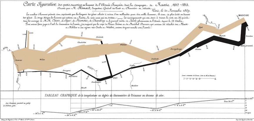
Minard’s Map of Napolean’s Russian Campaign of 1812

• Edward Tufte might say yes
• enormous amount of data laid out in organized, understandable fashion
• multi-media presentations of lines, numbers, pictures, narrative
• no proprietary platform, easily accessible by multiple users
• entirely content, e.g. no drop shadows, bullet indents etc…
• genuinely interactive (people instinctively look for familiar areas, etc…)

Minard’s Map Illustrates 6 principals (6 C’s) of analytic design and mapping (from Tufte)

• 1. comparisons, contrasts and differences
  • pre-post troop levels illustrated at beginning and end (started with 400K, ended with 10K)
• 2. causality and connections
  • path of retreating army tied to a temperature scale at bottom
• 3. complexity and multivariate data
  • six dimensions of data on the map: size of the army, location in lat and long, direction, temperature, places
• 4. cleverness, and innovative methods (use ‘whatever it takes’ to explain something)
  • map is annotated all over with numbers and words
• 5. credibility, by documenting the source of your data
  • two paragraphs at top are about sourcing and detail
• 6. content is king, tell a compelling story, ultimately stand or fall on the quality, integrity and relevance of your content
  • Minard’s map is essentially an anti-war poster telling a compelling story

Spatial Analysis

• See online presentation by Dave Unwin
• location as an explanatory variable
  • patterns in space, e.g. clustering
  • spatially varying risk
  • geographic or local covariates
• spatial data have additional structure
  • morphology - point, line, areal
  • geography - lat/long, CRS
  • attributes - elevation, population, measurements

R and Spatial Analysis

• familiar, unifying analytic environment
• many specialized packages and functions available
  • ability to translate most any spatial data
• rapidly incorporate advances
• growing, almost invariably supportive community

R spatial data

• spatial data frame - fundamental spatial R object
  • translates Cartesian coordinates to geography
• 3 important attributes
  • x/y become lat/long
  • Coordinate Reference System (CRS) relates lat/long to earth
  • “bounding box” to display the data

R spatial packages

• “base” packages - sp, maptools, rgdal
  • useful utilities to read in, transform, display, manipulate spatial data
• spatial statistics - gstat, geoR, spBayes
• areal data - spdep, DCluster, ade4, SpatialEpi
• point pattern data - spatial, splancs. spatstat

3 Basic Applications

• areal (or lattice) data
  • is there spatial variation?
  • if so, does pattern of spatial variation help explain why?
• point pattern data
  • are there clusters?
  • if so, does pattern help explain why?
• spatial interpolation
  • convert discrete observations to continuous fields
  • is the variable actually continuous, e.g. elevation, rain fall, temperature?
  • given a sample, what is the value at some non-measured location?

Areal Data: Suicide Mortality in 32 London Boroughs 1989-1993

• data from Congdon (2007) via Blangiardoa et al (2013)

• read in data

1
2
3
4
5
6
7
8
9
10
11
12
13
14
15
16

library(maptools)
library(spdep)

london<-readShapePoly("~ download ~ /LDNSuicides")
plot(london) # NB: no CRS
class(london)
names(london)
london$NAME

obs=c(75,145,99,168,152,173,152,169,130,117,124,119,134,90,
    98,89,128,145,130,69,246,166,95,135,98,97,202,75,100,
    100,153,194) # observerd number suicides each london borough
exp=c(80.7,169.8,123.2,139.5,169.1,107.2,179.8,160.4,147.5,
    116.8,102.8,91.8,119.6,114.8,131.1,136.1,116.6,98.5,
    88.8,79.8,144.9,134.7,98.9,118.6,130.6,96.1,127.1,97.7,
    88.5,121.4,156.8,114) # expected number suicides each london borough

• create dataframe of borough names, observed, expected
  • data is in alphabetical order, so have to sort the names from the spatial dataframe

1
2

NAME<- sort(london$NAME)
suicide.dat <- data.frame(NAME=NAME, obs=obs, exp=exp)

• calculate crude and empirical Bayes smoothed SMRS
  • NB: spdep tool probmap() calculates SMRs using population numbers

1
2
3
4

suicide.dat$SMR<-suicide.dat$obs/suicide.dat$exp

library(DCluster)
suicide.dat$smooth <- empbaysmooth(suicide.dat$obs,suicide.dat$exp)$smthrr

map the results

• reorder data file to match order in the spatial file

1
2
3

data.london<-attr(london,"data")
order<-match(data.london$NAME,suicide.dat$NAME)
suicide.dat<-suicide.dat[order,]

• establish and apply cut off values to categorize
• merge the smrs to spatial dataframe by name
• spplot to map

1
2
3
4
5
6

cuts<- c(0.6, 0.9, 1.0, 1.1,  1.8)
suicide.dat$SMR.cut<-cut(suicide.dat$SMR,breaks=cuts,include.lowest=TRUE)
suicide.dat$smooth.cut<-cut(suicide.dat$smooth,breaks=cuts,include.lowest=TRUE)
attr(london,"data")<-merge(data.london,suicide.dat,by="NAME")

spplot(london, c("SMR.cut", "smooth.cut"),col.regions=gray(3.5:0.5/4),main="")

• NB: Never use crude SMRS
  • In this example crude SMR’s are very close to smoothed
  • But this will generally not be so
  • crude SMRs are notoriously unstable and can be misleading…

Point Process Data: Broad Street Pump Cholera Outbreak

• What if John Snow had R?

load packages, read data (with rgdal), plot

• data from [Robin T. Wilson] (http://blog.rtwilson.com/john-snows-cholera-data-in-more-formats/)
• GDAL - geospatial data abstraction library
  • installation something of a bear…

1
2
3
4
5
6
7
8

library(spatstat)
library(rgdal)

cholera<-readOGR(" ~ download ~ /Cholera_Deaths.shp", "Cholera_Deaths")
pumps<-readOGR("~ download ~ /Pumps.shp", "Pumps")

plot(cholera, pch=16)
plot(pumps, add=T, col="red", pch=10, cex=3)

plot with background image

1
2
3
4
5
6

bkgrnd<-readGDAL(" ~ download ~ /Cholera_Deaths/SnowMap.jpg")

plot(cholera, pch=16)
image(bkgrnd,col = grey(1:99/100), add=T)
plot(cholera, pch=16, add=T, col="red")
plot(pumps, add=T, col="blue", pch=10, cex=3)

plot the point process with spatstat

• convert sp to ppp
• summarize and simple plot
• plot density comparing 2 bandwidths
  • overlay pump sites
• perspective plots
  • theta= option for view

1
2
3
4
5
6
7
8
9
10
11
12

cholera.point<-as.ppp(cholera)
summary(cholera.point)
plot(cholera.point)

plot(density(cholera.point,20))
plot(density(cholera.point,30))
plot(pumps, add=T, col="red", pch=10, cex=3)


persp(density(cholera.point,30))
persp(density(cholera.point,30), theta=90)
persp(density(cholera.point,30), theta=180)

Riply’s K statistic

• solid black line is observed K function
• dashed blue is expected

1
2

cholera.k<-Kest(cholera.point)
plot(cholera.k)

Spatial Interpolation

• Inverse Distance Weighting (IDW)
  • use neighboring samples to estimate every location on fine grid
  • gstat package - option “e=” controls degree of smoothing
  • results in ring contour lines
  • close to what surveyor might draw
  • but can’t assess error to externally validate
  • choice of smoothing exponent essentially arbitrary
  • clustered samples affect outcome
• variograms
  • estimate dependence between two points in space
  • distance on x-axis, semivariance on y axis
  • use to improve interpolations
• kriging
  • interpolation technique
  • incorporate variance for error estimates