COOKING A SAMPLE SIZE
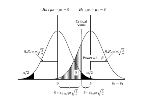
Difference between two groups on continuous measurement
Gerald van Belle “Statistical Rules of Thumb”
Andrew Gelman and Jennifer Hill’s “Data Analysis Using Regression and Multilevel/Hierarchical Models” (Chapter 20)
Brad Carlin
JoAnn Alvarez

Difference between two groups on continuous measurement

Difference between two groups on continuous measurement

Difference between two groups on continuous measurement

Difference between two groups on continuous measurement

Difference between two groups on continuous measurement

Difference between two groups on continuous measurement
Recognize denominator as the square of the standardized difference (\(\Delta ^2\)) \[ n_{group}=\frac{2(1.96 + 0.84)^2}{(\Delta)^2} \\ n_{group}=\frac{16}{(\Delta)^2} \]
10-point difference in IQ between two groups (mean population IQ of 100, and a standard deviation of 20): \[ n_{group}=\frac{16}{((100-90)/20)^2} \\ n_{group}=\frac{16}{(.5)^2} \]
total sample size of 128.
function in R
1 2 3 4 5 6 | |
1 2 3 | |
1 2 | |
1 2 3 4 | |
Rearrange Lehr’s equation to solve for the detectible standardized difference between two populations: \[ n_{group}=\frac{16}{(\Delta)^2} \\ (\Delta)^2 = \frac{16}{n_{group}} \\ \Delta = \frac{4}{\sqrt{n_{group}}} \\ \]
unstandardized difference \[ \delta = \frac{4 \sigma}{\sqrt{n_{group}}} \]
1 2 3 4 | |
1 | |
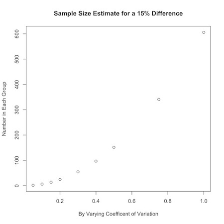
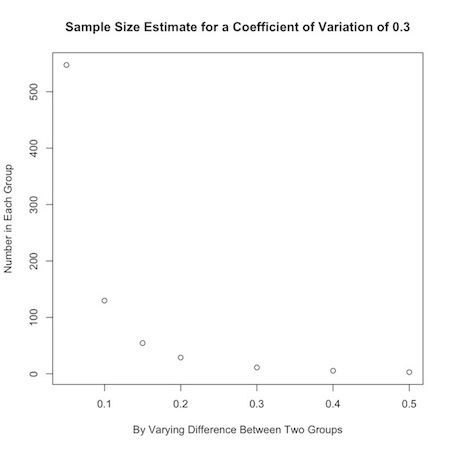
- \[ n_{group}=\frac{16(c.v.)^2}{(ln(\mu_0)-ln(\mu_1))^2} \\ n_{group}=\frac{16(c.v.)^2}{(ln(r.m.))^2} \]
R function
1 2 3 4 | |
1 2 3 4 5 6 | |
1 2 3 | |
- \[ y_i \sim Pois (\lambda) \\ \sqrt{y_i} \sim Nl(\sqrt{\lambda}, 0.25) \]
apply Lehr’s equation by taking the square root \[ n_{group}=\frac{4}{(\sqrt{\lambda_1}-\sqrt{\lambda_2})^2} \]
\(n_{group}=\frac{4}{(\sqrt{30}-\sqrt{36})^2} = 15\) units of observations in each group.
1 2 3 4 5 6 7 8 9 10 11 12 13 14 15 16 17 18 19 20 21 | |
Given no events or outcomes in a series of \(n\) trials, the 95% upper bound of the rate of occurrence \[ \frac{3}{n} \]
Set probability to statistical significance *\(1-0.95 = 0.05 = Pr[\Sigma y_1 = 0] = e^{n \lambda}\) *\(n \lambda = -ln(0.05) = 2.996\) *\(\lambda \approx 3/n\)
for RR *\(n_{group} = \frac{8(RR+1)/RR}{\frac{c}{c+d} (ln(RR))^2}\)
E.g. \(n_{group}=\frac{4}{(.3 - .1)^2} = 100\)
conservative approximation only valid where sample size each group between 10 and 100
For rare, discrete outcomes, you need at least 50 events in a control group, and an equal number in a treatment group, to detect a halving of risk.
incorporating uncertainty is inherently Bayesian
redefine basic Lehr’s formula R function in terms of difference and standard deviation.
1 2 3 4 5 | |
1 2 3 4 5 6 7 8 9 | |
can achieve same power under the same conditions with a few as 30 or as many as 160 observations in each group.
Power = \(\phi (\sqrt{\frac{n \theta ^2}{2 \sigma ^2}}-1.96)\)
1 2 3 4 5 | |
1 2 3 4 5 6 | |
use this info to define a Beta distribution to use as a prior in a binomial simulation
define parameters for Beta prior from mean and variance
1 2 3 4 5 6 7 | |
1 2 3 4 5 6 7 8 9 | |
if prior is \[ \theta \sim Beta(a,b) \]
and the likelihood is \[ X| \theta \sim Bin (N, \theta) \]
then the posterior is \[ \theta | X \sim Beta (X+a, N-X+b) \]
combines Binomial \({20 \choose 15} p^{15}q^{20-15}\) likelihood of external data with the \(Beta(9.2, 13.8)\),
1 2 3 4 5 6 7 | |
1 2 3 4 5 6 7 | |
1 2 3 4 5 6 7 8 9 10 11 12 13 14 15 16 | |
1 2 3 4 5 6 7 8 9 10 11 12 13 14 15 16 | |
now don’t hit 80% power until a sample size of about 54.
E.g. take the \(Beta(14+24.2,20-14+18.8)\) prior and shift 7 of the successes to failures as \(Beta(7+24.2,20-7+18.8)\)
1 2 3 4 5 6 7 8 9 10 11 12 13 14 15 16 | |