CONTINUOUS DATA ANALYSIS
Initial Approaches to Continuous Data: Means, Univariate, Boxplot
- Review, Clean, Familiarize
- missing values, unusual or incompatible values
- Descriptive Statistics *mean age, test results, e.g BP
- Establish Assumptions Met
- normally distributed? variance?
Review I
Normality
If your underlying population is normal, then the distribution of your sample means is also normal, and you can do things like calculate CI’s
the sample mean you are working with comes from a normally distributed population of all possible sample means so you can apply inferential statistics
Central Limit Theorem
- ROT ~ 30 data points
- Observational Epi ‘noiser’
Statistics
- \(Var=s^2 = \Sigma(x – \mu)^2 / n-1\)
- calculating formula \((\Sigma x^2 -(\Sigma x)^2/n)/n-1\)
- \(\sigma\) = \(\sqrt{s^2}\)
- \(c.v. = \sigma / \mu * 100\)
difference between \(\sigma\) and s.e.
- s.e. refers to the precision of an estimate
- \(\sigma\) refers to the variability of a sample, population or distribution itself
- CI contains true \(\mu\) x% of the time (true mean does not vary)
Useful %’s for Nl distn
- 68% data within 1 \(\sigma\)
- 95% data within 2 \(\sigma\)
- 99% data within 3 \(\sigma\)
PROC MEANS (review)
PROC MEANS data =  <options>;
VAR  variables;
RUN;
/* for example...*/
proc means data= your.data maxdec=4 n mean median std var q1 q2 clm stderr;
  var num_var;
  run;
- Defaults: #non-missing obs, mean, sd, min and max
Review II
skewness
- tendency to be more spread out on one side than the other
- right skewed- spread out on right side (positive skewness stat, mean > median)
- left skewed- spread out on left side (negative skewness statistic, mean < median)
- want skewness statistic close to zero, but can usually tolerate anything up to 1
kurtosis
- how peaked distribution is
- high peak, heavy tailed (leptokurtotic) positive statistics
- smaller peak, light tailed (platykurtic) negative statistic
- again want it close to zero (mesokurtotic)
quantiles
- value below which some proportion of the distribution lies
- quartile - 3 values divide a distribution into 4 equal parts
- Interquartile Range
- difference between first and third quartiles
- gives idea of how tightly clustered or spread out data is
- Boxplot - convenient graphical 5-number summary (mean, median, quartiles, minimum and maximum, outliers)
probability plots
- to see if a set of data is normally distributed
- plot your ordered data against their standardized values
- expect a straight line if data comes from a normal distribution
- single bend indicates skewness
- multiple curves indicates bi or multi modal distribution
- steps:
- order the data from low to high
- calculate the expected (normal) value for each observation
- plot Standard Normal points on your x axis vs. observed values on yaxis
PROC UNIVARIATE
PROC UNIVARIATE data =
       VAR num_var if no VAR, will analyze all variables;
        ID var  option so can id 5 lowest and 5 highest obs;
        HISTOGRAM num_var
        PROBPLOT  num_var
                goptions reset=all fontres=presentation ftext=swissb htext=1.5;
         /* options for the graph* /

/* e.g. */

proc univariate data = your.data mu0=n;
       var num_var;
        id idnumber;
        probplot num_var / normal (mu=est  sigma= est color=blue w=1);
        title;
run;
- more and varied defaults than PROC MEANS e.g. kurtosis, skewness
- more sophisticated graph options
- “plot” option returns stem and leaf plots, e.g.
2| 01189
3|1255568999
4|23
* “/normal” tells SAS to superimpose a reference line over plot
* also telling SAS to estimate mu and sigma from the data itself, and to make the line blue with a width of 1;
* “MU0” option for hypothesis testing (if you must)
* set mu0 to the null value youare interested in testing
PROC BOXPLOT
PROC BOXPLOT Data = ;
PLOT analysis var  group var  / options;
/* NB- data must be sorted by grouping var*/
RUN;


data work;
set work;
dummy = ‘1’;      /* creating dummy variable to do boxplot on just one group */
run;


proc boxplot data = work;
       plot cont_vardummy / boxstyle schematic  cboxes=black;
run;


symbol color = salmon;
   title ‘Nice Format Boxplot';
   proc boxplot data=work;
plot cont_varcat_var / cframe   = vligb
                       cboxes   = dagr
                       cboxfill = ywh;
run;
ANOVA AND LINEAR REGRESSION
ANOVA Using PROC GLM
- More flexible and powerful than PROC ANOVA
- allows us to easily create a data set of residuals for diagnostics testing
Review
ANOVA
- to compare >2 Means
- not appropriate to do multiple significance tests
- continuous response and categorical predictor
- F distribution
- ratio of two independent \(\chi^2\) divided by their d.f.’s
- \(\chi^2 = \Sigma (o-e)/e\)
- \(H_0\) two variances are equal
- divide larger variance by smaller (look up prob)
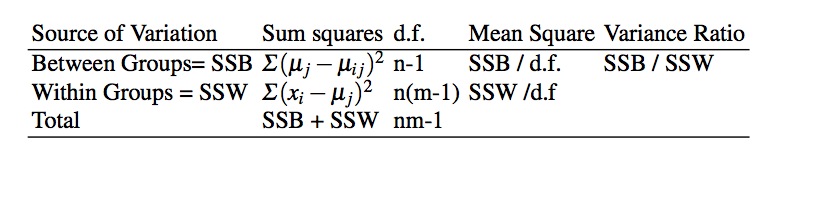
Sums of Squares
- \(TSS = SS_{Between} + SS_{Within}\)
- total = \(\Sigma\) (individual value - grand mean)
- between (model) = \(\Sigma\) (group mean - grand mean)
- estimate of the variance of the group means
- within (residual or error) = \(\Sigma\) (individual value - group mean)
- \(H_0\) no difference between the groups
- If true, then variance across groups, (SSB) should be (about) equal to to the variance within groups (SSW)
- F test measures this ratio (SSB/SSW)
- if between group variability is greater than within group variability, then assume groups are important
- The more F deviates from 1, the more significant the result
“Classic” ANOVA
- continuous response single categorical predictor
- basically comparing the means across 2 or more groups
- 2-sample t test is essentially a special case of ANOVA
assumptions
- independent observations
- continuously distributed outcome variable
- normal
- equal variances (homoscedasticity)
are your data consistent with assumptions?
proc univariate data = your data;
     class cat_var;
     var cont_var;
     probplot cont_var / normal  (mu=est sigma=est color=blue w=1);
     title ‘univariate analysis by categorical variable’;
run;


proc sort data=your.data out=sorted_data; /* need to sort data by your  categorical variable* /
    by cat_var
run;

proc boxplot data=sorted_data;
       plot cont_varcat_var  / cboxes=black boxstyle=schematic;
run;
- normality
- PROC MEANS, UNIVARIATE and BOXPLOT
- CLASS statement in PROC UNIVARIATE to categorize data (get descriptive statistics across groups) *homoscedasticity
- Levene’s Test of Homogeneity (SAS ‘hovtest’)
Using error terms to test assumptions
another view of ANOVA
- Outcome = Overall AVG + Differential Effect CAT + Error
- Where outcome assumed ~Nl r.v. with equal variances across groups
- NB: error term is the only r.v. on the R side of the equation
- Equal to the outcome r.v. on left side of equation (plus 2 constants)
- Must also be ~Nl r.v. with equal variances across groups
- much easier to test our assumptions of normality on the pooled error terms (especially in multiple regression).
error terms
- aka Residuals
- denoted by \(r\) or \(\hat{e}\)
- difference between the observed value and that predicted by the model
- (should be) random, normally distributed, average=0
- We will feed them into PROC UNIVARIATE and PROC GPLOT to test our assumptions
PROC GLM
PROC GLM  data =    ;
      CLASS  grouping variables
      MODEL  specify the model i.e. response variable = predictors
      MEANS computes means for each group
      LSMEANS to test specific group differences
      OUTPUT (out =) creates output data set of residuals
RUN;
QUIT;  /*note, GLM is like GPLOT need to end it or remains invoked */


/* SYNTAX TEMPLATE */
options ls=75 ps=45;  /* page and line spacing options*/
PROC GLM data = your.data;
       CLASS cat_var;
       MODEL num_var=cat_var;
       MEANS cat_var / hovtest;
       OUTPUT out=check r=resid   p=pred;  /* creating an output data
set called ‘check’ in which ‘r ‘ is a keyword SAS recognizes as
residuals and ‘p’ recognized as predictors */
title ‘testing for equality of means with GLM’;
RUN;
QUIT;


/* now run gplot on the ‘check’ dataset created above*/

PROC GPLOT data=check;
         PLOT residpred / haxis=axis1 vaxis=axis2 vref=0; /* can
leave out if ok with  defaults*/
         axis1 w=2 major=(w=2) minor=none offset=(10pct);
         axis2 w=2 major=(w=2) minor=none;
         TITLE ‘plot residuals vs predictors for cereal’;
RUN;
QUIT;

/* now run proc univariate to get histogram, normal plot, kurtosis and skewness on residuals*/

PROC UNIVARIATE data = check normal;
      VAR resid;
      HISTOGRAM / normal;
      PROBPLOT/ mu=est sigma=est color=blue w=1;
      TITLE;
RUN;
GLM ANOVA Output
- administrative info
- variable chosen as the class variable, how many levels in the class,
- number of observations and how many of those observations were used inthe analysis
- ANOVA table
- model=between
- error=within
- sums of squares
- F = model (between) ss / error (within) ss (converted to a p value)
- \(R^2\) = model ss / total ss
- Model ‘fit’
- coefficient of variation = Root MSE / weight Mean
Finding the Group(s) that differ(s)
Caution experiment-wise vs. comparison-wise error rate
- Side-by-Side Comparison of Boxplots
- Significant F Test in ANOVA
- unequal group means
- Adjust experiment-wise error rate
- LSMEANS –request multiple comparison table
- ADJUST = TUKEY controls for all possible comparisons
- divides \(\alpha\) by # all possible comparisons
- ADJUST = BONFERRONI controls for pre-planned comparisons
- divide \(\alpha\) by # planned comparisons
- NB: ADJUST=T does not invoke TUKEY
- requests individual t –tests
- not recommended
Requesting GLM Multiple Comparisons
PROC GLM data=your.data;
   CLASS cat_var;
   MODEL cont_var=cat_var;
   LSMEANS cat_var / pdiff=all adjust=tukey; /*adjust=bon*/
   /* pdiff=all requests all pairwise p values */
TITLE ‘Data: Multiple Comparisons';
RUN;
QUIT;
- Interpretation of output
- order the means, e.g. 1<3<4<2
- If a pair of means is not significantly different, draw a line under it
- remaining comparisons are important
Accounting for More than 1 Categorical Variable: n-Way ANOVA and Interaction Effects
Example: do different levels of a drug have differing effect on different diseases?
\[
y_{ijk} = \mu + \alpha_i + \beta_j + (\alpha \beta)_{ij} + \epsilon_{ijk}
\]
where
\(y_{ijk}\) is the observed blood pressure for each subject
\(\mu\) is the overall population mean blood pressure
\(\alpha_i\) is the effect of disease \(i\)
\(\beta_J\) is the effect of drug dose \(j\)
\((\alpha \beta)_{ij}\) interaction term between disease \(i\) and dose \(j\)
\(\epsilon_{ijk}\) is the residual or error term for each subject
- Outcome variable is drug effect on BP
- Two categorical explanatory variables:
- Drug Dose
- Pre-Existing Disease
- Interaction Term…
- the condition where the relationship of interest is different at different levels (i.e. values) of the extraneous variables (Kleinbaum Kupper, Muller and Nizam)
- here drug dose and disease type.
- diseases A,B,C * doses 1,2,3,4 = 12 possible outcomes
Syntax for n-Way ANOVA
/* Pre-ANOVA PROC MEANS*

proc means data=sasuser.b_drug mean var std;
   class disease drug;
   var bloodp;
   title 'Selected Descriptive Statistics for drug-disease
combinations';
run;


/* Means Plot To Illustrate Results*/

proc gplot data=sasuser.b_drug;
   symbol c=blue w=2 interpol=std1mtj line=1;/* interpolation method
gives s.e. bars */
   symbol2 c=green w=2 interpol=std1mtj line=2;
   symbol3 c=red w=2 interpol=std1mtj line=3;
   plot bloodpdrug=disease; / vertical by horizontal /
   title 'Illustrating the Interaction Between Disease and Drug';
run;
quit;

/*Syntax for Interaction Term*/

proc glm data=sasuser.b_drug;
   class disease drug;
   model bloodp=disease drug diseasedrug;/note interaction
term/
   title 'Analyze the Effects of Drug and Disease';
   title2 'Including Interaction';
run;
quit;


/* LSMEANS Syntax with Interaction */
/* must look at all combinations of drug and disease*/

proc glm data=sasuser.b_drug;
   class disease drug;
   model bloodp=drug disease drugdisease;
   lsmeans diseasedrug / adjust=tukey pdiff=all; /note looking at
combinations/
   title 'Multiple Comparisons Tests for Drug and Disease';
run;
quit;
A Look at Interaction in Epidemiology
(See DiMaggio Chapter 11, section 6…)
CORRELATION with PROC CORR
Pearson correlation coefficient
\(r = \Sigma (x_i - \bar{x}) * (y_i - \bar{y}) / \sqrt{\Sigma(x_i - \bar(x)^2 * (\bar{y})^2)}\)
- to quantify linear relationships
- sum of products about the mean of 2 variables divided by the square root of their sum of squares
- relationships can be +, - or none
- Correlation does not mean causation
- plot the data first
PROC CORR Syntax
PROC CORR DATA=work rank;  /* ‘rank’ orders
                                correlations from high to low */
        VAR predictor1 predictor2 predictor3 predictor4
        WITH outcome_var;
        TITLE ‘correlation of outcome with predictors’;
RUN;

/*to get a correlation matrix,
  omit the ‘with’ statement */
SIMPLE LINEAR REGRESSION with PROC REG
Regression
\[
y=\beta_0 + \beta_1 x + \epsilon
\]
Where,
\(\beta_0\) is the outcome when the predictor \(x\) is 0
\(\beta_1\) is the slope (the `rise over the run’), or amount of change in the outcome \(y\) per unit change in the predictor \(x\)
\(\epsilon\) error term (defined as it was with ANOVA)
Method of Least Squares
\(\hat{\beta_0} = \bar{y} - \hat{\beta_1} \bar{x}\)
\(\hat{\beta_1} = \Sigma(x_i-\bar{x})(y_i-\bar{y}) / \Sigma(x_i-\bar{x})^2\)
- best fitting line, close as possible, on average, to all the data points
- minimize deviation of distance from the line to the data points in the y direction
- confidence interval around \(\hat{\beta_1}\) is \(\hat{\beta_1}\) \(t_{\alpha/2, n-2} * se(\hat{\beta_1})\)
- hypothesis test for \(\hat{\beta_1}\) is \(\hat{\beta_1}/ se(\hat{\beta_1})\) compared to critical value \(t_{\alpha/2, n-2}\)
- null hypothesis no relationship between x and y
- mean or average value (\(\hat{y}\)) will give us more or better information about y than x does
- analogous to the model\(H_0: \beta_1=0\), test that the slope of the regression line is not statistically significant from zero.
Analysis of Variance Perspective
Total Variability (TSS) Distance from Data Points to Mean Line: \(\Sigma (y_i-\bar{y})^2\)
Explained Variability (SSM) Distance from Regression Line to Mean Line: \(\Sigma(\hat{y}-\bar{y})^2\)
Unexplained Variability (SSE) Distance from Data Points to Regression Line: \(\Sigma(y_i-\hat{y})^2\)
As in ANOVA, if it’s a good model, we expect more explained than un-explained variability and the proportion of the total variability explained by our regression model to be closer to 1:
Assumptions
- same as ANOVA:
- linearity
- True underlying linear relationship
- Look at scatterplots
- normality
- At any give value of predictor (x) outcome (y) is nl
- homogeneity of variance
- y also has same variance for any value of x
- independence
Residuals
- histograms and normal plots
- plot residuals against the predictor variables
- expect uniform distribution within 2 s.e.’s of 0.
- Data points beyond 2 s.e.’s may be outliers
- tests for influential values
- patterns may indicate deviation from assumptions
- possible need to transform data
PROC REG
PROC REG DATA=work;
          MODEL cont_outcome_var = cont_pred_var;
          TITLE ‘simple linear regression’;
RUN;
QUIT; / need to quit out of the procedure /
Other tools in SAS will give regressions, but PROC REG is convenient with rich set of tools
Basically a call to PROC REG and a model statement
Proc Reg Output
- general approach
- over-all p first
- then individual t tests for the predictors
- then \(R^2\) for explained variance
- Model SS = Explained (Between) SS
- Error SS = Unexplained (Within)
- F = Explained / Unexplained
- p value – associated with F statistic
- H0 is that the model does not fit i.e. x is not statistically significantly linearly related to Y, i.e. B1 = 0
- Parameter estimates:
- \(\beta_0\) intercept, may not be relevant
- \(\beta_1\) slope of predictor variable
- Both with p values
- Can plug into equation
- Note, for simple linear regression \(t = \sqrt{F}\)
Producing predicted values:
- Could (if you wanted) do it by hand
- Easier to let SAS do it
- create a temporary data set with the values you want predictions for
- append those values to the data set you used to create the model
- calculate the values by specifying ‘p’ (for ‘predict) option in the model statement
Multiple Regression in PROC REG
- \(H_0\): dependent variable (y) doesn’t change based on \(x_i\)
- No longer a single line
- 2 predictors = plane
- Increased complexity
- Good because most processes are complex
- But…..difficult to determine which model ‘best’
- Basic modeling (and assumptions) remains the same
- Complex relationships Residuals!
- Questions to ask:
- Is the overall model significant?
- Based on What?
- Are the individual predictors significant?
- Why or why not?
Dummy Variables
- Linear regression intended for numeric variables
- Numbers have meaning. 2 is twice 1. 50 is ten times 5.
- Categorical variables don’t make sense to REG
- Solution is Dummy Variables
- Have only 2 values: 0, 1
- E.g. male/ not male, poor / not poor
- If > 2 levels, need additional dummy variables
- E.g. 3 levels, needs 2 dummy variables
- mild, moderate, severe
- moderate / not moderate, severe / not severe
- ‘mild’ is the referent category
REGRESSION DIAGNOSTICS
Common Problems in Linear Regression
- Collinearity
- Outliers and Influential observations
- Non-constant variance (heteroscedasticity)
- Non-independent (correlated) errors
- Non-normality
Residual Plots
- helps uncover problems with our assumptions
- residual = difference between predicted and actual values
- unexplained variance in our model
- plot residual value on y-axis
- independent (predictor) variable value on x-axis
- Check residuals for a mean of 0 at each value of the predictor variable
- random scatter around a reference line of zero
- normally distribution at each value of the predictor variable
- the same variance at each value of the predictor variable (independence)
- Residual Plot Patterns
- U-shaped non-linearity
- Funnel-shaped heteroscedasticity
- Sine-shaped non-linearity, violation of normality, non-independence, time-series effect
Outliers and Influential Values
- use PROC REG (easier than GLM)
- plot the residuals vs. the predicted values
- Include all the predictors
- look for gross violations
- if potential problem look for pattern that mimics it in the individual predictor plots
Studentized Residuals
- Residuals divided by standard error
- absolute value less than 2 occurred by chance
- between 2 and 3 are infrequent (<5%)
|3| rarely occur by chance alone
Jacknife Residual (RSTUDENT)
- Difference between studentized residual with and without the possible outlier
- remove potential outlier and plot the difference between the observed value and the prediction line with and without the outlier
- If RSTUDENT different from STUDENT for that observation, it is likely to be influential
Cook’s D Statistic
- change in parameter estimate after deleting observation
- suggested cut off D > 4/n (n=sample size)
- printed out for every observation in data set
Requesting Residuals Plots in SAS
plot r.  p.
/* SAS recoginizes r. and p. as referring to residuals and predictors*/

plot student.  obs.
/* SAS recognizes student. as studentized residual and obs. as* observation number /

plot student.  nqq.
/* nqq. refers to normal quantile values, another name for a normal probability plot */

/* example syntax*/

options ps=50 ls=97;

goptions reset=all fontres=presentation ftext=swissb htext=1.5;


PROC REG data=fitness;
MODEL oxygen_consumption = runtime age run_pulse maximum_pulse;
   PLOT r.(p. runtime age run_pulse maximum_pulse); /*plot residuals vs. predicted values */
   PLOT student.obs. / vref=3 2 -2 -3     /* studentized obs. Gives obs. # to ID */
                        haxis=0 to 32 by 1;
   PLOT student.nqq.; /nqq another name for normal prob plot/
   symbol v=dot;
   TITLE ‘Plots of Diagnostic Statistics';
RUN;
QUIT;
Requesting Outlier Statistics in SAS
/* MACRO FOR OUTLIERS */

/*  set the values of these macro variables, */
/*  based on your data and model.            */
%let numparms=5;  /* # of predictor variables + 1 */
%let numobs=31;   /* # of observations */
%let idvars=name; /* relevant identification variable(s) */

data influential;
   set ck4outliers;
   cutcookd=4/&numobs;

   rstud_i=(abs(rstud)>3);
   cookd_i=(cooksd>cutcookd);
   sum_i=rstud_i + cookd_i;
   if sum_i > 0;
run;

/* then print out the list of influential observations */

proc print data=influential;
   var sum_i &idvars cooksd rstud cutcookd
       cookd_i rstud_i;
   title 'Observations that Exceed Suggested Cutoffs';
run;
- ‘r’ option after model statement returns studentized residuals (STUDENT) and Cook’s D
- ‘influence’ option after model statement returns Jackknife residual (RSTUDENT)
How to handle influential observations:
- Don’t just throw them out
- Check data and correct errors
- Build a better model or collect more data
- Consider an interaction term or higher order terms e.g. squares of age etc…
Collinearity: Variance Inflation Factor
- \(VFI_i = 1 / (1-R^2_i)\)
- for the variable \(X_i\), \(R^2_i\) is the \(R^2\) value from a regression with \(X_i\) (normally a predictor variable) set as the outcome or dependent variable
- e.g. if the model is \(Y = \beta_0+\beta_1X_1+\beta_2 X_2+\beta_3 X_3 +\beta_4X4\), , we calculate \(R^2_3\) for \(X_3\) by fitting the model \(X3 = \beta_0+\beta_1X_1+\beta_2 X_2\) .
- higher R2 for a predictor, the smaller the denominator and the larger the VIF
- VIF > 10 indicates collinearity
About Model Building
SAS Automated Methods
- “/ SELECTION =” model option in PROC REG
- RSQUARE, ADJRSQ (e.g. “/ selection=adjrsqr”)
- Tests all possible combinations (k var = \(2^k\) models)
- FORWARD
- Run all single predictor models, keep significant ones, then run all 2-predictor models, etc…
- BACKWARD
- Run model with all var, drop one at time, selecting significant models at each step
- STEPWISE
- Hybrid, start with none, add most significant single, if var becomes non-sig, drop it
Problems with automated approach
- Strictly based on p values
- SAS default p values too high (0.1 to 0.5)
- multiple significance testing
- different model from each method
- do not take important causal concepts such as confounders, mediators into account
Sample Automated Selection Syntax
PROC REG data=work.data;

  Forward:  model outcome=pred1 pred2 pred3 / SELECTION=FORWARD
SLENTRY=0.001;

  Backward:  model outcome=pred1 pred2 pred3 / SELECTION=BACKWARD
SLENTRY=0.001;

  Stepwise:  model outcome=pred1 pred2 pred3 / SELECTION=STEPWISE
SLENTRY=0.001;
Other (Better) Approaches to Model Building
- Causal thinking should drive analysis …
- Analysis does not drive causal thinking …
- basics work
- univariate analyses, plot data, stratified analyses, diagnose outliers, assess fit
- try partial F-tests
Partial F-test
- overall F-test: \(H_0\): all regression coefficients zero
- partial F test: does the addition of any specific independent variable, given others already in the model, significantly contribute to the prediction of Y?
- e.g. how much a variable, x, contributes to a model given that variables \(x_1\), \(x_2\) etc… are already in the model.
- extra SS [x | x1, x2…xp ] = model SS [ x1, x2…xp + x] - model SS [ x1, x2…xp ]
- test \(H_0\) ‘addition of x to a model already containing \(x_1\), \(x_2\) etc…does not significantly improve the prediction of Y
- compute F [x | x1, x2…xp ] = SS [x | x1, x2…xp ] / model ss [x1, x2…xp + x]
Using partial F-tests in SAS
model  y = a b c d
/ TEST c=0 d=0
- tests joint significance of c and d given that a and b are in the model
- Type I ss = ‘sequential sum of squares’
- When var added in particular sequence
- Type II ss = ‘variable added last sum of squares’
- Assumes all other variables have been added
Introducing Logistic Regression
Why Logistic Regression
PROC MEANS data=lbw;
CLASS smoke;
VAR low;
RUN;
- Epidemiologists are very interested in dichotomous outcomes
- ill vs. not ill
- injured vs. non-injured
- dead vs. alive
- Linear regression doesn’t handle dichotomous outcomes very well
- what does the mean of a 0/1 variable mean?
- Dichotomous outcomes violate assumptions of linearity, homoscedasticity and normality
PROC LOGISTIC
PROC LOGISTIC DATA = lbw DESCENDING;
    MODEL low = smoke / RL;
    RUN;
    QUIT;
- DESCENDING modeling probability of y = 1
- RL requests 95% CI for parameter estimates
- 1 unit increase in predictor associated with a \(\beta\) increase in log odds of outcome
- exponentiate to get odds ratio
- ratio of two odds
- e.g. \(\beta\) for smoking 0.6931
- exp(0.6931) = 1.999906
why exponentiation results in odds ratios
- log odds low birth weight smokers
- \(-1.0985 + 1 * 0.6931 = -0.4054\)
- log odds low birth weight non-smokers
- \(-1.0985 + 0 * 0.6931 = -1.0985\)
- odds for smokers
- \(exp(-0.4054) = 0.6667101\)
- odds for non-smokers
- \(exp(-1.0985) = 0.3333708\)
- odds ratio
- \(0.6667101/0.3333708 = 1.999906\)
some options for proc logistic
PROC LOGISTIC DATA = work.data DESCENDING;
    CLASS categorical.var / param=ref ref=first;
    *CLASS categorical.var (ref="rich") / param=ref ref=first;
    MODEL dichot.outcome = categorical.var num.var / RL;
    UNITS num.var=SD
RUN; QUIT;
- Param=ref: tells SAS to use reference coding for all variables in the CLASS statement
- Ref = first: Global option telling SAS to use the first level of all classification variables as reference
- Ref= last can also be used
- SD requests standard deviation of indep var to be unit
- SD gives the beta coeff. for a 1 SD decrease in indep var