INTRODUCTION TO BAYESIAN ANALYSIS FOR EPIDEMIOLOGISTS

What is Bayes?

• “the explicit use of external evidence in the design, monitoring, analysis, interpretation and reporting of a (scientific investigation)” (Spiegelhalter, 2004)

• A Bayesian is one who, vaguely expecting to see a horse and catching a glimpse of a donkey, strongly concludes he has seen a mule. (Senn, 1997)

• “You shall know them by their posteriors”

Acknowledgements

Jim Albert
David Spiegelhalter and Nicky Best
Andrew Gelman

THE BAYESIAN WAY

Why Bayes?

• natural and coherent
• now not only theoretically correct, but practical and doable
• advantages
  • flexible (adapt to each situation)
  • efficient (uses all available information)
  • intuitively informative (provides relevant quantitative summaries)
    • the way we think and learn
    • combine what you observe (data) and what you believe

Basics of Bayes

• prior distribution (\(Pr[\theta]\)) reflects beliefs
  • \(\theta\) is a random variable, it has a probability distribution which reflects our uncertainty about it
    
• likelihood (\(Pr[y|\theta]\)) reflects data
  • model for the probability of observing the data
• posterior distribution (\(Pr[\theta|y]\)) combining beliefs and data
  • We use Bayes theorem : \[ posterior \; \propto \; prior \; * \; likelihood \\ p(\theta | y) \propto p(\theta)*p(y | \theta) \]
  • expressing uncertainty about parameters with probability distributions (revolutionary)

There is no free lunch

• To get a reasonable probability distribution out, need
  • reasonable opinions about the plausibility of values
  • tune the computational “machinery”
  • test sensitivity to models and distributions

Contrast with frequentist approaches

• Frequentist
  • parameters are fixed or non-random
  • assume the effect is 0 (\(H_0\))
  • determine what the trial tells us about the treatment effect
• Bayesian
  • State the plausibility of different values of the treatment effect (the prior distribution)
  • State the support for different values of the effect based solely on the trial data (the likelihood)
  • Combine these two sources to produce a final opinion about the treatment effect (the posterior distribution)
  • learn whether the trial should change our opinion about the treatment effect

Bayes Theorem

• know \(Pr[A|B]\) can get at \(Pr[B|A]\)

• derivation \[ Pr[A \cap B] = Pr[B \cap A] \\ Pr[A \cap B] = Pr[A|B] Pr[B]\\ Pr[B \cap A] = Pr[B|A] Pr[A]\\ Pr[A|B] Pr[B] = Pr[B|A] Pr[A]\\ Pr[A|B] = \frac{Pr[B|A] Pr[A]}{Pr[B]}\\ Pr[B|A] = \frac{Pr[A|B] Pr[B]}{Pr[A]} \]

• by law of total probability, \(Pr[A] = Pr[A|B] Pr[B] + Pr[A|\overline{B}] Pr[\overline{B}]\)

• so denominator, \[ Pr[B|A] = \frac{Pr[A|B] Pr[B]}{Pr[A|B] Pr[B] + Pr[A|\overline{B}] Pr[\overline{B}]}\\ Pr[B|A] = \frac{Pr[A|B] Pr[B]}{\sum Pr[A|B] Pr[B]} \]

• for continuous probability distributions, \[ Pr[B|A] = \frac{Pr[A|B] Pr[B]}{\int dB Pr[A|B]Pr[B]} \]

• or (n terms of parameters and data) \[ Pr[\theta|y] \frac{Pr[y|\theta] Pr[\theta]}{\int dB Pr[y|\theta]Pr[\theta]} \]

• note, all denominator does is make sure integrates to total probability of 1, i.e. normalizing factor
• concentrate on the numerator, which is proportional to \(p(y|\theta)p(\theta)\)
  • same form, just the size changes.

HIV, ELISA, Western Blot

• sensitivity of ELISA
  • \(Pr[+|D]\)
  • calculation \[ \frac{Pr[D|+]P[+]}{Pr[D|+]P[+] + Pr[D|-]P[-]}\\ \frac{(498/502)(502/1000)}{(498/502)(502/1000) + (10/498)(498/1000)} \]

• In R: \(((498/502)*(502/1000))/(((498/502)*(502/1000)) + ((10/498)*(498/1000)))\) = 98%

• positive predictive value \[ Pr[D|+] = \frac{Pr[+|D]P[D]}{Pr[+|D]P[D] + Pr[+|\overline{D}]P[\overline{D}]}\\ = \frac{(498/508)(508/1000)}{(498/508)(508/1000) + (4/488)(492/1000) } \]

• 99%.

different population, different prevalence, different prior

• positive predictive value \[ \frac{(1960/2000)(2000/1000000)}{(1960/2000)(2000/1000000) + (784/998000)(998000/1000000)} \]

• 20%.

• a frequentist is someone who only uses Baye’s Theorem sometimes

Example: Student Sleep Habits

• what proportion of college students who get more than 8 hours sleep?
• believe about 30%.
• survey says 11 of 27 (47%)

• the Rev. Bayes says \[ posterior \; \propto \; prior \; * \; likelihood \\ p(\theta | y) \propto p(\theta)*p(y | \theta) \]

• binomial likelihood (data) \(\theta^k * (1-\theta)^{n-k}\)
  • \(\theta\) probability sleeping > 8 hours
  • \(k\) number positive responses
  • \(n\) sample size
• discrete prior
  • plausible values for proportion of heavy sleepers (theta)
    • 0.05, 0.15, 0.25, 0.35, 0.45, 0.55, 0.65, 0.75, 0.86, 0.95
  • weights for those plausible values
    • 0, 1, 2, 3, 4, 2, 1, 0, 0, 0
  • convert to probabilities
    • 0.00, 0.08, 0.15, 0.23, 0.31, 0.15, 0.08, 0.00, 0.00, 0.00
• calculate the posterior
  • multiply each value of posterior by likelihood of that value
  • calculations involve log transformations
    • LearnBayes function pdisc()

R Code for Student Sleep Example

• assign likelihood data to object, create prior, plot

1
2
3
4
5
6

data<-c(11, 16)  # number successes and failures

theta<-seq(0.05, 0.95, by = 0.1)
weights<-c(0, 1, 2, 3, 4, 2, 1, 0, 0,0)
prior<-weights/sum(weights)
plot(theta, prior, type="h", ylab="Prior Probability")

• use pdisc() to calculate posterior, print a table

1
2

post<-pdisc(theta, prior, data) 
round(cbind(theta, prior, post), 2) 

• plot how prior changed when consider data

1
2
3
4
5
6
7

library(lattice) 
PRIOR=data.frame("prior",theta,prior) 
POST=data.frame("posterior",theta,post) 
names(PRIOR)=c("Type","Theta","Probability") 
names(POST)=c("Type","Theta","Probability") 
data=rbind(PRIOR,POST) 
xyplot(Probability~Theta|Type,data=data,layout=c(1,2), type="h",lwd=3,col="black")

PROBABILITY DISTRIBUTIONS USED IN BAYESIAN ANALYSIS

• flexible distributions
  • the form changes based on parameters

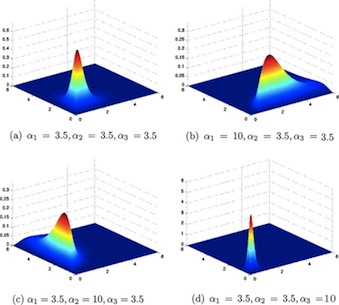
The Normal Distribution

\[ \sim Nl(\mu, \sigma^2) \]

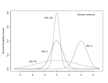
The Normal Distribution

• continuous variables or parameters
• dnorm(mean, precision)
  • NB precisions, \(1/\sigma^2\)
  • flat prior, very large variance, very small precision
  • dnorm(0,.0001) , dnorm(0,1.0E-4).
• half-normal to restrict
  • dnorm(0,1.0E-4)I(0,)

The Uniform Distribution

\[ \sim Unif(a,b), \\ \mu = \frac{(a+b)}{2}, \\ \sigma^2 = \frac{(b-a)^2}{12} \]

The Uniform Distribution

• dunif(a,b)
• only take values on interval (a,b)
  • standard deviations, oproportion parameters on the interval (0,1)
• “flat prior”, set large range e.g. dunif(-100,100) or dunif(0,100) for positive parameters

The Exponential Distribution

\[ \sim Exp(\lambda),\\ mu=1/\lambda,\\ \sigma^2=1/\lambda^2 \]

The Exponential Distribution

• likelihood positive continuous variables, e.g. time to events
• prior for Beta-distributed parameters
  • “flat prior”, set lambda to be small, eg dexp(.01)

The Gamma Distribution

\[ \sim \Gamma(\alpha, \beta),\\ \mu=\frac{\alpha}{\beta} \\ \sigma^2=\frac{\alpha}{\beta^2} \]

The Gamma Distribution

• more general case of the exponential
• \(\alpha\) “shape” parameter, \(\beta\) “scale” parameter.
• \(\alpha=1\) results is an exponential distribution (\(\mu=1/\beta\)).
  
• \(\sim \Gamma(\alpha/2, 1/2)\) is \(\chi^2\) with \(\alpha\) d.f.
• for positive continuous variables, counts, time to events
• prior for normal precision terms, Beta parameters
• dgamma(alpha, beta)
• small \(\alpha\) and \(\beta\), eg dgamma(.001,.001), for “flat” prior

The Beta Distribution

\[ \sim Beta(\alpha,\beta)\\ \mu=\frac{\alpha}{\alpha+\beta}\\ \sigma^2=\frac{\alpha \beta}{(\alpha \beta)^2 (\alpha + \beta) + 1} \]

The Beta Distribution

• returns values between 0 and 1
• often used to model proportions and probabilities
• \(\alpha\) successes, \(\beta\) failures
• conjgate to binomial distribution likelihood
• set \(\alpha\) and \(\beta\) equal to 1 for flat prior
• set \(\alpha > 0\) and \(\beta > 0\) forproper distribution that can be integrated
• set \(\alpha > 1\) \(\beta > 1\) for unimodal distribution
• \(\alpha, \beta \to \infty\), distribution approaches normality.
• dbeta(alpha, beta)

The Dirichlet Distribution

\[ \sim Dirichlet(\alpha_1, ... \alpha_k) \]

The Dirichlet Distribution

• extension of the Beta distribution
  • for several probability parameters that must sum to 1
• for multinomial proportions or probabilities
  • take values between 0 and 1
• ddirch(alpha[])
  • \(\alpha_i\) is vector of number of outcomes of type i
• flat prior, set alpha as a vector of 1’s: c(1,1,….,1)

CONJUGATE ANALYSIS

What is Conjugate Analysis?

• statistical relationship between the prior, the likelihood and the posterior distribution.
• prior is conjugate to a likelihood if both the prior and the posterior are in the same statistical “family”
• e.g. binomial likelihood conjugate to Beta posterior
• until relatively recently (advent of MCMC) essentially all Bayesian analysis was conjugate
  • BUGS and JAGS still use it if convenient closed form available
• don’t exist for all likelihoods

Conjugate Analysis of Proportions

• interested in \(p\), proportion of some outcome
  • generically refer \(\theta\)
• likelihood or \(Pr(y | \theta)\)
• k responses out of n patients
• follows binomial probability distribution, \(\binom{n}{k} p^k q^{n-k}\)
  • \(p\) probability of the event occurring in a single trial,
  • \(q\) probability of the event not occurring (\(1-p\) by the complement rule)
• \(\binom{n}{k}\) binomial expansion ’’n choose k"
  • \(\frac{n!}{k!(n-k)!}\)
• prior for \(\theta\)
  • our beliefs before we see data
  • e.g., uniform prior, all values equally likely
    • \(\sim Unif(0,1)\)
    • \(Pr(\theta)\) is then \(1/1+0=1\)
• posterior
• Bayes’ Theorem \[ Pr(\theta|y) = Pr(\theta | k, n) \propto (\theta^k)(1-\theta)^{n-k}*1 \]
  • note, proportionality rather than equality, avoiding the often problematic normalizing denominator

• conjugate solution with our prior \[ \sim Beta(1+k, 1+n-k) \]

• conjugacy binomial and beta \[ Beta(a+k,b+n-k) \]

• e.g. student sleep habits
• 11 of 27 sleep more than 8 hours
• assume Beta(1,1) prior
• Beta(1+11, 1+38-11) = Beta(12, 28) posterior

• in R, sample the beta distribution * x<-rbeta(1000, 12,28) plot(density(x)) summary(x)

Drug Response Example: No Data

• plan a trial of 20 patients what is the probability that 15 will respond?

• believe drug is about 40% patients effective
  • may vary between 20% and 60%
  • sd about 10%
• Beta(9.2,13.8) fits this prior
  • will talk about how to get this in a moment

• monte carlo simulation in BUGS or JAGS

1
2
3
4
5
6

Model{
y~dbin(theta , 20)         #sampling distribution
theta ~ dbeta (9.2, 13.8)  #parameter from sampling distribution
p.crit <- step(y-14.5)     # indicator variable, 1 if y>=15, 0 otherwise
}

• or code it up in R

1
2
3
4
5
6
7
8
9

N=1000
theta<-rbeta(N,9.2,13.8)
x<-rbinom(N,20, theta)
y<-0
accept<-ifelse(x>14.5, y+1, y+0)
prob<-sum(accept)/N
prob
library(coda)
densityplot(accept)

• answer is pure Monte Carlo
• draw samples or simulate from a distribution
• no data from actual patients in this example (yet)

Drug Response Example: Data

• run the trial
  • enroll and treat 20 volunteers and 15 of them respond
• now interested in effectiveness of drug given the data
  • can use conjugate analysis

• prior still Beta (9.2, 13.8)

• but now have a likelihood

• binomial probability of 15 successes in 20 trials

• posterior with conjugate approach
  • Beta (9.2+15, 13.8+20-15) = Beta (24.2, 18.8)
• “Bayesian” learning
  • take Beta (9.2, 13.8) probability distribution (prior)
  • combine with Binomial probability distribution of the 15 successes in 20 trials data (likelihood)
  • to update the Beta prior as our posterior
• probability of 25 successes in additional 40 patients?
• “update” the analysis
• Beta-Binomial posterior from previous analysis becomes new prior
  • 95% tail probability of new posterior is 0.3

MCMC of Drug Example

• what if there was no convenient, closed conjugate solution?
• Markov Chain Monte Carlo

• algorithms to evaluate posterior given (almost) any prior and likelihood

• write the model in code form

• write the model code.

1
2
3
4
5
6
7
8
9

cat(
"model
{
y~dbin(theta, m) #likelihood
theta~dbeta(a,b) # prior
y.pred~dbin(theta, n)  #posterior, used as predictive distribution
p.crit<- step(y.pred-ncrit+0.5) # if y.pred>=ncrit, returns 1, otherwise 0  
}"
,file="m1.jag")

• specify the data
  • beta parameters
  • number of trials

1
2
3
4
5
6

m1.dat<-list(a=9.2,
b=13.8,
y=15,
m=20,
n=40,
ncrit=25)

• initialize stochastic nodes
  • beginning values for random draws for \(\theta\)
  • both BUGS and JAGS will do this for you
  • better to do it yourself
• here single value for single series of draws (“chain”)

1

m1.inits<-list(theta=0.1)

• use R2jags
  • interface for JAGS
    • convenient, cross-platform (vs. Win/OpenBUGS)
  • rjags object
  • can convert to mcmc (or any other R) object

1
2
3
4
5
6
7
8
9
10
11
12
13
14

library(R2jags)

m1<-jags(data=m1.dat, n.chains=1,
    inits=m1.inits, 
    parameters.to.save=c("theta", "p.crit"), 
    model.file="m1.jag")

class(m1)
print(m1)
plot(m1)
traceplot(m1)

m1.mcmc<-as.mcmc(m1)
plot(m1.mcmc)

• simulation results same (or very close) to closed, conjugate result

Beta Parameters from mean and standard deviation

1
2
3
4
5
6
7

estBetaParams <- function(mu, var) {
  alpha <- ((1 - mu) / var - 1 / mu) * mu ^ 2
  beta <- alpha * (1 / mu - 1)
  return(params = list(alpha = alpha, beta = beta))
}

estBetaParams(.4,(.1)^2)

• posted on StackExchange
• or can use beta.select() from LearnBayes

Conjugate Analysis of Normally Distributed Data

• see THM Concentration example on website

Conjugate Binomial Analysis

• see placenta previa example on website

Conjugate Analysis of Count Data

• Poisson likelihood \[ P(k) = e^{-\lambda} * \lambda^k / k \]

• \(\mu = \sigma^2 = \lambda\)

• conjugate Gamma(a,b) prior
  • \(\mu = \frac{a}{b}\)
  • \(\sigma^2 = \frac{a}{b^2}\)
• \(Gamma(a+n\bar{x}, b+n)\) posterior
  • posterior mean \(\frac{a+n\bar{x}}{b+n}\)
  • compromise between prior mean (\(\frac{a}{b}\)) and MLE mean (\(\bar{x}\))

London Bombings During WWII

• number of bomb hits in \(36km^2\) area of South London during World War II
  • partitioned into \(0.25km^2\) grid squares:
• 537 events (\(\Sigma x_i * n_i=537\) total hits)
• 576 observations (\(\Sigma n_i=576\) areas)

• mean \(\bar{x}=537/576=0.93\)

• Poisson likelihood with hit rate \(\theta = \lambda\)
• “invariant” Jeffreys prior (will will discuss this later)
  • \(p(\theta) \propto \frac{1}{\sqrt{\theta}}\)
  • equivalent to an (improper) Gamma (0.5, 0)

• posterior \[ p(\theta | y) = \Gamma(a+n\bar{x}, b+n) = \Gamma(537.5, 576) \\ \mu = 537.5/ 576 = 0.933 \\ \sigma^2 = 537.5/ 576^2 = 0.0016 \]

• again, posterior mean is compromise between prior mean and the MLE
• s.d. is less than each of prior s.d. and the MLE s.d.

• as sample size increases, posterior mean approaches MLE mean, posterior s.d. approaches MLE s.d.

Heart Transplant Mortality

• interested in heart transplant 30-day mortality as “success”
  • mortality data for target hospital and peer institutions

• model as Poisson process of counts

• likelihood (data) for target hospital \(y_t \sim Pois(\mu, e \lambda_t)\), where
  • \(y_t\) = observed # deaths
  • \(n_t\) = # surgeries
  • e = expected # deaths
  • \(\lambda_t\) = risk of death
• MLE for \(\lambda_t\) is \(\frac{observed}{expected}\) = \(\frac{y}{e}\)
  • poor estimator
    • expected number (denominator) very small
    • variance is appreciably larger than the mean

• Bayesian approach can be informative.

• Gamma prior conjugate to Poisson likelihood
  • \(\Gamma(\alpha, \beta)\) prior for \(\lambda\)
  • base prior on peer institutions
  • number deaths (\(y_c\)), number surgeries (\(n_c\)), in peer hospitals to define the \(\alpha\) and \(\beta\) terms Gamma prior for \(\lambda\)
  • \(\Gamma(\Sigma y_c, \Sigma n_c)\) prior
    • based on \(p(\lambda) \propto \lambda{\alpha-1}*e{-\beta \lambda}\)

• posterior \[ \Gamma(\alpha + y_t, \beta + n_t ) = \Gamma(\Sigma y_c + y_t, \Sigma n_c + n_t ) \]

• compare two hospitals
  • hospital A, 1 death in 66 surgeries
  • hospital B, 4 deaths in 1767 surgeries
  • comparison group 10 peer hospitals, 16 deaths in 15,174 surgeries
• unadjusted MLE estimates
  • 1.5% (95% CI 0.08%, 9.3%) hospital A
  • 0.2% (95% CI 0.07%, 0.6%) hospital B

1
2
3
4
5
6
7
8
9
10
11
12
13

y_A<-1
n_A<-66
prop.test(y_A, n_A)


y_B<-4
n_B<-1767
prop.test(y_B, n_B)


y_T<-16
n_T<-15174
prop.test(y_T, n_T)

• define and sample posterior distributions
  • conjugate relationship

1
2

lambda_A<-rgamma(1000, shape=y_T+y_A, rate=n_T+n_A)
lambda_B<-rgamma(1000, shape=y_T+y_B, rate=n_T+n_B)

• summarize and plot the comparison

1
2
3
4
5
6
7
8
9
10
11
12

summary(lambda_A)
summary(lambda_B)

t.test(lambda_A, lambda_B)

par(mfrow = c(2, 1)) 
plot(density(lambda_A), main="HOSPITAL A", xlab="lambda_A", lwd=3) 
curve(dgamma(x, shape = y_T, rate = n_T), add=TRUE) 
legend("topright",legend=c("prior","posterior"),lwd=c(1,3)) 
plot(density(lambda_B), main="HOSPITAL B", xlab="lambda_B", lwd=3) 
curve(dgamma(x, shape = y_T, rate = n_T), add=TRUE) 
legend("topright",legend=c("prior","posterior"),lwd=c(1,3))

• not very different
  • statistical significance due to n
• plots: prior more influence on hospital A
  • because hospital A has less data